Orbit Independent Solution: The Universal Anomaly

You may have noticed that the equations for the ellipse and the hyperbola are quite similar. In many cases, they differ only by a negative sign or a change from circular to hyperbolic trigonometric functions. This is largely due to the fact that all of the orbits are conic sections, so they share a similar mathematical genealogy.

The equations for an ellipse and a hyperbola are summarized in Table 2.

Table 2 The equations representing the ellipse and hyperbola trajectories

Equation	Ellipse (\(e < 1\))	Hyperbola (\(e > 1\))
Orbit equation (true anomaly)	\(r = \frac{h^2}{\mu} \frac{1}{1 + e\cos\nu}\)	\(r = \frac{h^2}{\mu} \frac{1}{1 + e\cos\nu}\)
Cartesian Coordinates	\(\frac{x^2}{a^2} + \frac{y^2}{b^2} = 1\)	\(\frac{x^2}{a^2} - \frac{y^2}{b^2} = 1\)
Semimajor axis	\(a = \frac{h^2}{\mu}\frac{1}{1 - e^2}\)	\(a = \frac{h^2}{\mu}\frac{1}{e^2 - 1}\)
Semiminor Axis	\(b = a\sqrt{1 - e^2}\)	\(b = a\sqrt{e^2 - 1}\)
Energy Equation	\(\frac{v^2}{2} - \frac{\mu}{r} = -\frac{\mu}{2a}\)	\(\frac{v^2}{2} - \frac{\mu}{r} = \frac{\mu}{2a}\)
Mean anomaly	\(M_e = \frac{\mu^2}{h^3}\left(1 - e^2\right)^{3/2}t\)	\(M_h = \frac{\mu^2}{h^3}\left(e^2 - 1\right)^{3/2}t\)
Kepler’s Equation	\(M_e = E - e \sin E\)	\(M_h = e\sinh F - F\)
Orbit equation (eccentric anomaly)	\(r = a\left(1 - e\cos E\right)\)	\(r = a\left(e\cosh F - 1\right)\)

The Universal Variable

Since these equations are so similar, we will try to find a way to unify them, such that we can solve a single equation regardless of the type of orbit. Given the initial position and velocity of the orbiting mass, we can determine the semimajor axis of the orbit from the energy equation:

(245)\[a = \left(\frac{2}{r_0} - \frac{v_0^2}{\mu}\right)^{-1}\]

Notice that for a hyperbolic orbit, \(a\) will be negative from this equation, in contrast to our previous definition where \(a\) was positive. This gives an easy way of determining the type of orbit before finding the eccentricity.

Then, we will define the universal variable, or universal anomaly \(\chi\), which is by definition zero at \(t_0\) (the time when \(\vector{r}_0\) and \(\vector{v}_0\) are known). This is analogous to the true anomaly, which is zero on the apse line, and we previously defined \(t_0\) to occur at the apse line.

Using the universal anomaly, we can find the position and velocity of the orbiting mass at any future time via:

(246)\[\begin{split}\begin{aligned}\vector{r} &= \left[1 - \frac{\chi^2}{r_0}C\left(\alpha\chi^2\right)\right]\vector{r}_0 + \left[\left(t - t_0\right) - \frac{\chi^3}{\sqrt{\mu}}S\left(\alpha\chi^2\right)\right]\vector{v}_0\\\vector{v} &= \frac{\chi\sqrt{\mu}}{r r_0}\left[\alpha\chi^2S\left(\alpha\chi^2\right) - 1\right]\vector{r}_0 + \left[1 - \frac{\chi^2}{r}C\left(\alpha\chi^2\right)\right]\vector{v}_0\end{aligned}\end{split}\]

where \(\alpha = 1/a\) and we will define \(C(z)\) and \(S(z)\) shortly. Note that \(\alpha < 0\) for hyperbolas, \(\alpha = 0\) for parabolas (\(a\rightarrow\infty\)) and \(\alpha > 0\) for ellipses. This gives \(\chi\) dimensions of square root of length, such that \(\alpha\chi^2\) is dimensionless.

In a previous section, we identified the coefficients of \(\vector{r}_0\) and \(\vector{v}_0\) in equations similar to (246) as the Lagrange coefficients, in that case, in terms of the change of true anomaly. Eqs. (246) give the Lagrange coefficients in terms of the universal anomaly.

Now, we need a way to solve for \(\chi\), the universal anomaly. We can write Kepler’s equation in terms of the universal anomaly as:

(247)\[\sqrt{\mu}\left(t - t_0\right) = \frac{r_0 v_{r,0}}{\sqrt{\mu}}\chi^2 C\left(\alpha\chi^2\right) + \left(1 - \alpha r_0\right) \chi^3S\left(\alpha\chi^2\right) + r_0 \chi\]

Like Kepler’s equation in the ellipse and hyperbola specific forms, this equation is transcendental in \(\chi\). If \(\chi\) is known, the equation can be solved for the change in time interval, \(t - t_0\). If the time interval is known instead, we must use numerical techniques to solve the equation.

Next, we need to define the functions \(C(z)\) and \(S(z)\).

Stumpff Functions

The functions \(C(z)\) and \(S(z)\) are Stumpff functions. They can be defined by infinite series of the form:

(248)\[c_k(z) = \frac{1}{k!} - \frac{z}{\left(k + 2\right)!} + \frac{z^2}{\left(k + 4\right)!} - \cdots = \sum_{i=0}^{\infty}\frac{\left(-1\right)^{i} z^i}{\left(k + 2i\right)!}\]

where \(k\) is an integer that indicates the type of Stumpff function.

To solve Eq. (247), we don’t want to work with the infinite series forms of the Stumpff equations. Instead, we will convert the Stumpff functions to trigonometric functions using the Taylor series expansions of the circular and hyperbolic trigonometric functions. The first third and fourth Stumpff functions, \(k=2\) and \(k=3\) respectively, define our \(C(z)\) and \(S(z)\) functions from above.

(249)\[\begin{split}C(z) =\begin{cases}\displaystyle \frac{1 - \cos\sqrt{z}}{z} & \left(z > 0\right)\\ \displaystyle\frac{\cosh\sqrt{-z} - 1}{-z} & \left(z < 0\right) \\ \displaystyle\frac{1}{2} & \left(z = 0\right)\end{cases}\end{split}\]

and

(250)\[\begin{split}S(z) =\begin{cases}\displaystyle \frac{\sqrt{z} - \sin\sqrt{z}}{\left(\sqrt{z}\right)^3} & \left(z > 0\right)\\ \displaystyle \frac{\sinh\sqrt{-z} - \sqrt{-z}}{\left(\sqrt{-z}\right)^3} & \left(z < 0\right) \\ \displaystyle \frac{1}{6} & \left(z = 0\right)\end{cases}\end{split}\]

The two Stumpff functions are plotted in Fig. 59. Notice that both \(C(z)\) and \(S(z)\) tend toward infinity as \(z\) approaches \(-\infty\), and they approach zero as \(z\) approaches \(+\infty\).

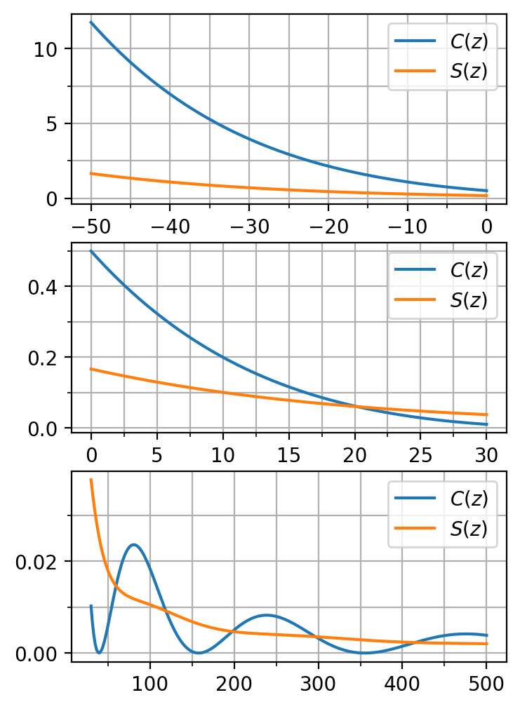
Fig. 59 The Stumpff functions defined by Eqs. (249) and (250). Note the varying \(x\) axes on the plots.

Relation of \(\chi\) to Other Anomalies

We now seek to relate \(\chi\) back to the anomalies for elliptical, parabolic, and hyperbolic orbits. For demonstration, we will choose the following initial conditions:

(251)\[t_0 = 0\quad r_0 = r_p \quad v_{r,0} = 0\]

which is to say, the same initial conditions that we defined for the equations in terms of the true and eccentric anomalies. For the case of the parabola, \(\alpha = 0\) and we can show that:

(252)\[M_p = \frac{1}{6}\left(\frac{\chi\sqrt{\mu}}{h}\right)^3 + \frac{1}{2}\left(\frac{\sqrt{\mu}}{h}\chi\right)\]

In the case of the ellipse, we know that \(\alpha > 0\), and we can show that:

(253)\[M_e = \frac{\chi}{\sqrt{a}} - e \sin\left(\frac{\chi}{\sqrt{a}}\right)\]

Finally, for the hyperbola, \(\alpha < 0\) and \(a < 0\), and we can show that:

(254)\[M_h = e\sinh\left(\frac{\chi}{\sqrt{-a}}\right) - \frac{\chi}{\sqrt{-a}}\]

Summarizing these results, the universal anomaly \(\chi\) is related to our previously defined anomalies as follows:

(255)\[\begin{split}\chi =\begin{cases}\displaystyle\frac{h}{\sqrt{\mu}}\tan\frac{\nu}{2} & \text{parabola} \\\displaystyle\sqrt{a}E & \text{ellipse} \\\displaystyle \sqrt{-a}F & \text{hyperbola}\end{cases}\end{split}\]

Generalizing from this to the case where \(t_0\neq 0\), and does not occur at periapse, we find:

(256)\[\begin{split}\chi =\begin{cases}\displaystyle\frac{h}{\sqrt{\mu}}\left(\tan\frac{\nu}{2} - \tan\frac{\nu_0}{2}\right) & \text{parabola} \\\displaystyle\sqrt{a}\left(E - E_0\right) & \text{ellipse} \\\displaystyle \sqrt{-a}\left(F - F_0\right) & \text{hyperbola}\end{cases}\end{split}\]

where \(\nu_0\), \(E_0\), and \(F_0\) are the true anomaly and eccentric anomalies at the time \(t_0\).

Numerical Solution of Kepler’s Equation in the Universal Anomaly

To formulate the numerical solution of Kepler’s equation in terms of the universal anomaly, we move everything over to one side of the equation, and seek the roots of:

(257)\[f(\chi) = 0 = \frac{r_0 v_{r,0}}{\sqrt{\mu}}\chi^2 C\left(\alpha\chi^2\right) + \left(1 - \alpha r_0\right) \chi^3S\left(\alpha\chi^2\right) + r_0 \chi - \sqrt{\mu}\left(t - t_0\right)\]

The derivative of this function is also useful:

(258)\[\begin{split}\begin{multline} \frac{d f(\chi)}{d\chi} = 2\frac{r_0 v_{r,0}}{\sqrt{\mu}}\chi C(z) + \frac{r_0 v_{r,0}}{\sqrt{\mu}}\chi^2 \frac{d C(z)}{dz} \frac{dz}{d\chi} \\ \qquad+ 3\left(1 - \alpha r_0\right)\chi^2 S(z) + \left(1 - \alpha r_0\right)\chi^3 \frac{d S(z)}{dz}\frac{dz}{d\chi} + r_0 \end{multline}\end{split}\]

where \(z = \alpha\chi^2\), such that:

(259)\[\frac{dz}{d\chi} = 2\alpha\chi\]

and

(260)\[\begin{split}\begin{aligned}\frac{d S(z)}{dz} &= \frac{1}{2z}\left[C(z) - 3S(z)\right] \\\frac{d C(z)}{dz} &= \frac{1}{2z}\left[1 - z S(z) - 2C(z)\right]\end{aligned}\end{split}\]

Substituting these results back into Eq. (258) gives:

(261)\[\frac{d f(\chi)}{d\chi} = \frac{r_0 v_{r,0}}{\sqrt{\mu}}\chi\left[1 - \alpha\chi^2 S(z)\right] + \left(1 - \alpha r_0\right)\chi^2 C(z) + r_0\]

The last thing we need for a solution using Newton’s algorithm is an initial guess. There are several methods suggested for this. In [Cur20], they suggest using:

(262)\[\chi_{i = 0} = \sqrt{\mu} \left\lvert\alpha\right\rvert \Delta t\]

In [PC13], they suggest a couple of different options. First, Prussing and Conway show that the solution lies in the interval:

(263)\[\begin{split}\begin{aligned}\chi^{+} &= \frac{\sqrt{\mu}\Delta t}{r^{-}}\\\chi^{-} &= \frac{\sqrt{\mu}\Delta t}{r^{+}}\end{aligned}\end{split}\]

where \(r^{+}\) and \(r^{-}\) are the largest and smallest values of the radius. The most conservative choice of \(r^{-}\) is the radius at periapsis for all the orbits:

(264)\[r^{-} = r_p\]

For elliptical orbits, the most conservative choice of \(r^{+}\) is the radius at apoapse:

(265)\[r^{+}_{\text{ellipse}} = r_a\]

For parabolas and hyperbolas, the most conservative choice is \(r^{+} = \infty\), such that:

(266)\[\chi^{-}_{\text{parabola/hyperbola}} = 0\]

With values of \(\chi^{+}\) and \(\chi^{-}\) computed, the initial guess is simply the average of the two:

(267)\[\chi_{i = 0} = \frac{\chi^{+} + \chi^{-}}{2}\]

Alternatively, a more refined estimate can be determined using a secant estimate of the root of Kepler’s equation:

(268)\[\chi_{i = 0} = \frac{\mu\Delta t^2}{r_p \left[f(\chi^{+}) + \sqrt{\mu}\Delta t\right]}\]

where \(f(\chi^{+})\) is the solution of Kepler’s equation with the \(\chi^{+}\) value.

Note

Prussing and Conway [PC13], citing Conway [Con86] suggest that faster convergence in the solution of Kepler’s equation can be achieved by using the Laguerre algorithm, rather than Newton’s algorithm. Another advantage of the Laguerre algorithm is that it is relatively insensitive to the value of the initial guess.

The Laguerre algorithm can be implemented as:

(269)\[\chi_{i + 1} = \chi_{i} - \frac{n f(\chi_i)}{f'(\chi_i) \pm \left[\left(n - 1\right)^2 \left(f'(\chi_i\right)^2 - n\left(n - 1\right) f(\chi_i)f''(\chi_i)\right]}\]

The sign ambiguity in the denominator is determined by taking the sign of the numerical value of \(f'(\chi_i)\). In addition, the solution is relatively insensitive to the choice of the value of \(n\), which is an integer constant. It seems as though \(n = 5\) is a reasonable value. Choosing \(n = 1\) gives the standard Newton’s algorithm.

Derivation of \(f''(\chi_i)\) is left up to the reader.

Although the Laguerre algorithm was originally intended for finding the roots of polynomial equations, it seems to work well in this application.