Plane Change Maneuvers

So far, all the orbital maneuvers we have considered have been coplanar—the initial and final orbits shared the same inclination relative to the orbital focus. However, this need not be the case, and we will relax that assumption in this section.

In particular, orbital plane changes are necessary in many cases when the launch location does not match the desired orbit. Since the latitude of the launch location affects the orbital inclination, achieving certain orbits requires an orbital plane change depending on the launch latitude. One example is geosynchronous equatorial orbit (\(i\) = 0°). If the spacecraft is launched from anywhere except the equator, a plane change is required to change the inclination.

Analysis of Plane Change Maneuvers

We will consider plane changes that have a common focus for the initial and target orbits. For a transfer to occur with a single impulse, the orbital planes must intersect and the intersection of two planes forms a line. Since the orbits have the same focus, the line of intersection of the planes must pass through the focus.

Due to the geometry of this maneuver, it is most convenient to use a coordinate system attached to the moving spacecraft. The unit vectors are parallel and perpendicular to the position vector from the focus. Thus, the velocity is given by:

(310)\[\vector{v} = v_r \uvec{u}_r + v_{\perp} \uvec{u}_{\perp}\]

This is shown in Fig. 68.

Fig. 68 A single-impulse plane change maneuver. The orbital planes intersect at a line through the focus of the orbit. Transfer is possible between the orbits by rotating the velocity vector of the spacecraft around the radial vector. Note that the radial velocity magnitude may change, as shown here, but the direction remains the same.

For a single impulse maneuver, there are up to two locations on the line of intersection where the maneuver can be performed. The plane rotation takes place around the line of intersection. For an impulsive maneuver, the position of the spacecraft doesn’t change.

Therefore, the radial velocity does not change direction during a plane change maneuver, although it may change magnitude. This is shown in Fig. 68. In other words, if orbit 1 is the initial orbit and orbit 2 is the target, we can say:

(311)\[\uvec{u}_{r,1} = \uvec{u}_{r,2} = \uvec{u}_r\]

Fig. 69 The plane change maneuver from Fig. 68 shown looking down the line of intersection. The circle at the intersection of the orbits represents the focus of the orbits. The radial velocity vector is projecting out of the screen.

The plane change is accomplished by changing the direction of the perpendicular velocity component. The angle between the initial and final perpendicular components of the velocity is the dihedral angle, \(\delta\). This is shown on Fig. 69. Like the radial velocity, the perpendicular velocity may also change its magnitude during a plane change maneuver.

Required Change of Velocity

The vector change in velocity for a plane change maneuver is found by:

(312)\[\Delta\vector{v} = \vector{v}_2 - \vector{v}_1 = \left(v_{r,2} - v_{r,1}\right)\uvec{u}_r + v_{\perp,2}\uvec{u}_{\perp,2} - v_{\perp,1}\uvec{u}_{\perp,1}\]

The magnitude of the velocity change is found by taking the dot product of \(\Delta\vector{v}\) with itself:

(313)\[\Delta v^2 = \Delta\vector{v}\cdot\Delta\vector{v} = \left(v_{r,2} - v_{r,1}\right)^2 + v_{\perp,2}^2 + v_{\perp,1}^2 - 2v_{\perp,1}v_{\perp,2}\left(\uvec{u}_{\perp,1}\cdot\uvec{u}_{\perp,2}\right)\]

The last term, the dot product of the two azimuthal unit vectors \(\uvec{u}_{\perp}\), can be replaced by the product of their magnitudes (which is unity) and the cosine of the angle between them, so we obtain:

(314)\[\Delta v^2 = \left(v_{r,2} - v_{r,1}\right)^2 + v_{\perp,2}^2 + v_{\perp,1}^2 - 2v_{\perp,1}v_{\perp,2}\cos\delta\]

There are four terms in this equation that can be changed by the maneuver. To keep \(\Delta v\) at a minimum for a given dihedral angle \(\delta\):

1. The radial velocity component should be constant, so that \(v_{r,2} - v_{r,1} = 0\)

2. The perpendicular velocity should be as small as possible

This occurs when the initial and target orbit intersect at their apoapsis. If the maneuver occurs at apoapsis, the radial velocity component will be zero in both orbits, \(v_{r,2} = v_{r,1} = 0\). In addition, the azimuthal velocity components will be the smallest on the orbit. From Eq. (310) with \(v_{r} = 0\), \(v_1 = v_{\perp,1}\) and \(v_2 = v_{\perp,2}\), so Eq. (314) reduces to:

(315)\[\Delta v = \sqrt{v_1^2 + v_2^2 - 2v_1v_2\cos\delta}\]

In Terms of Flight Path Angle

If the maneuver does not occur at apoapsis, then we need to use Eq. (314) to find \(\Delta v\). However, it may be more convenient to work with the velocity magnitude and the flight path angle, rather than the two velocity components. In that case, since:

(316)\[\begin{aligned} v_r &= v \sin\phi & v_{\perp} &= v \cos\phi \end{aligned}\]

where \(\phi\) is the flight path angle, Eq. (314) becomes:

(317)\[\Delta v^2 = v_1^2 + v_2^2 - 2 v_1 v_2\left[\cos\Delta\phi - \cos\phi_2\cos\phi_1\left(1 - \cos\delta\right)\right]\]

If \(\delta\) = 0° and there is no plane change, then this equation reduces to the same equation we developed previously for non-Hohmann transfer trajectories, Eq. (300).

Pure Rotation of the Orbital Plane

In some cases, it may only be necessary to rotate the orbital plane, without changing any of the other orbital elements. If there is no speed change, only a change of direction of the velocity vector, then \(v_1 = v_2 = v\). By using the trigonometric identity:

(318)\[\cos\delta = 1 - 2\sin^2\frac{\delta}{2}\]

and setting \(v_1 = v_2 = v\) (that is, no speed change), Eq. (314) for \(\Delta v\) reduces to:

(319)\[\Delta v_{\delta} = 2v\sin\frac{\delta}{2}\]

where the subscript \(\delta\) indicates this is for pure rotation of the orbital plane.

By dividing both sides of this equation by \(v\), we can plot the relative \(\Delta v\) versus \(\delta\). On Fig. 70, a value of \(\Delta v / v\) of 1.0 means that the \(\Delta v\) required is equal to the spacecraft speed, whatever that happens to be.

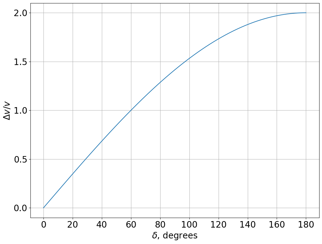
Fig. 70 The required velocity increment as a function of dihedral angle for pure rotation maneuvers.

As we can see from Fig. 70, plane change of about 24° requires the same \(\Delta v\) as is needed to increase the speed to the escape velocity from a circular orbit, \(\Delta v / v \approx\) 0.414.

Similarly, a plane change of 60° requires a \(\Delta v\) equal to the current spacecraft velocity! In LEO, the velocity is approximately 7.5 km/s. A plane change of 60°, with an \(I_{sp}\) of 300, would require over 90% of the spacecraft mass to be propellant.

This is why plane changes are often described as very expensive maneuvers, that should be avoided whenever possible once a spacecraft is in orbit. Instead, plane changes should be accomplished during launch. During launch, significantly more propellant can be provided for much less cost, since it does not have to be lifted all the way to orbit.

Launch Azimuth

In some cases, however, plane changes are unavoidable due to the latitude of the launch site of the spacecraft. One common example is putting a spacecraft in geosynchronous equatorial orbit. It is not possible to launch a spacecraft into an equatorial orbit unless the launch site is on the equator.

We know that the orbital plane must intersect with the center of the earth. Therefore, if a spacecraft is launched from any latitude above or below the equator, the orbit will have some natural inclination relative to the equatorial plane.

The final inclination of the orbit can also be controlled by determining the launch azimuth. The launch azimuth is the flight direction when the spacecraft is inserted into its orbit. It is equal to 0° pointing North and increases clockwise. Therefore, launches due East have an azimuth of 90°, due South of 180°, and due West of 270°.

A launch azimuth of 90° (due East) takes most advantage of the rotation of the earth to give a velocity boost to the spacecraft. Since the orbital speed is relative to the inertial coordinates fixed to the earth’s center, launching in an eastward direction reduces the \(\Delta v\) required to achieve a particular orbital speed.

The linear velocity at the equator is the ratio of the earth’s circumference and its sidereal period:

(320)\[v_{\text{equatorial}} = 2 \pi R_E/\omega_E = 2\pi \cdot \unit{6378}{km} / \unit{23.9345}{h} = \unit{0.4651}{km/s}\]

The velocity at any latitude can be found by multiplying this by the cosine of the latitude:

(321)\[v_{\text{latitude}} = v_{\text{equatorial}} \cos\phi\]

The due East launch azimuth also puts the spacecraft into an orbit with its inclination equal to the launch latitude. The relationship between launch azimuth, latitude, and orbital inclination is given by:

(322)\[\cos i = \cos\phi\sin A\]

where \(A\) is the launch azimuth.

For northeasterly (\(0° < A < 90°\)) and southeasterly (\(90° < A< 180°\)) launch azimuths, the spacecraft does not take full advantage of the earth’s rotational velocity. These launch azimuths produce an inclination greater than the launch latitude, but less than 90°. Since these orbits have a velocity component in the eastward direction, they are called prograde orbits.

Launches to the west, with \(180° < A < 360°\), are called retrograde orbits. These produce an inclination between 90° and 180°.

To produce an inclination of 90° requires a launch due North or due South, respectively. These are the polar orbits.

Fig. 71 shows a plot of the orbital inclination obtained for a range of latitudes and launch azimuths. We can see that the only way to achieve an inclination of 0° or 180°, an equatorial orbit, is to launch from the equator (\(\phi\) = 0°) with a launch azimuth of \(A\) = 90° (due East) to make a prograde orbit or \(A\) = 270° (due West) for a retrograde orbit.

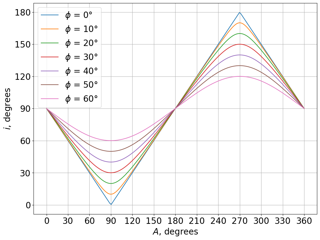
Fig. 71 The launch azimuth, \(A\), in combination with the latitude \(\phi\) determines the inclination of the orbit after launch.

Practical Launch Azimuth Considerations

As a practical consideration, launch azimuths are limited by the geography surrounding the launch site. Launches from Kennedy Space Center in Florida (\(\phi\)=28.6°N) are limited to azimuths between 35° and 120° so that they do not cross land over the US. Therefore, polar orbits (\(i\) = 90°) are not possible to achieve from Kennedy.

BokehDeprecationWarning: 'tile_providers module' was deprecated in Bokeh 3.0.0 and will be removed, use 'add_tile directly' instead.

BokehDeprecationWarning: 'get_provider' was deprecated in Bokeh 3.0.0 and will be removed, use 'add_tile directly' instead.

Fig. 72 The permitted launch angles from Kennedy Space Center on the East coast of the US. The vertical line indicates due north/south. The upper line indicates the maximum northerly launch azimuth while the lower line indicates the maximum southerly launch azimuth.

The other major launch site in the US is Vandenberg Space Force Base in southern California (\(\phi\) = 34.7°N). Similar restrictions at Vandenberg require most launches to go to the south, over the Pacific Ocean. However, polar and sun-synchronous orbits are possible from Vandenberg, where the azimuth limits are from 158° to 201°.

BokehDeprecationWarning: 'get_provider' was deprecated in Bokeh 3.0.0 and will be removed, use 'add_tile directly' instead.

Fig. 73 The permitted launch angles from Vandenberg Space Force Base on the Wast coast of the US. The vertical line indicates due north/south. The upper line indicates the maximum northerly launch azimuth while the lower line indicates the maximum southerly launch azimuth.