Example: Elliptical Orbit

A geocentric elliptical orbit has a perigee radius of 9600 km and an apogee radius of 21,000 km. Calculate the time to fly from perigee to a true anomaly of \(\nu =\) 120°. Then, calculate the true anomaly 3 hr after perigee.

Given True Anomaly, Find Time Since Perigee

The three steps of the solution procedure when we are given \(\nu\) and want to find \(t\) are:

1. Calculate the eccentric anomaly, \(E\), from the true anomaly, \(\nu\)

2. Calculate the mean anomaly, \(M_e\), from the eccentric anomaly

3. Calculate the time since periapsis, \(t\), from the mean anomaly

To complete these steps, we require two other orbital elements besides the true anomaly:

1. eccentricity, \(e\)

2. semimajor axis, \(a\)

Let’s find \(e\) first, since it is the only orbital element that appears in Eq. (203) to find \(E\). We can find \(e\) directly using Eq. (140), repeated here for reference:

\[e = \frac{r_a - r_p}{r_a + r_p}\]

import numpy as np
from scipy.optimize import newton

mu = 3.986004418E5  # km**3/s**2

r_p = 9_600  # km
r_a = 21_000  # km
nu_1 = np.radians(120)
e = (r_a - r_p)/(r_a + r_p)

The eccentricity of this orbit is \(e =\) 0.3725. Then, the eccentric anomaly found from Eq. (203) is:

E_1 = 2 * np.arctan(np.sqrt((1 - e)/(1 + e)) * np.tan(nu_1 / 2))

The eccentric anomaly is \(E_1 =\) 1.73 radians. The subscript 1 indicates this is the first part of this example.

Now, to find the time to fly to the true anomaly of 120°, we need to find \(M_e\). This is done with Kepler’s equation, Eq. (204).

M_e1 = E_1 - e * np.sin(E_1)

The mean anomaly is \(M_{e,1} =\) 1.36 radians. Finally, calculating the time from the mean anomaly requires the period.

a = (r_a + r_p) / 2
T = 2 * np.pi / np.sqrt(mu) * a**(3 / 2)
t_1 = M_e1 * T / (2 * np.pi)

The semimajor axis of the orbit is \(a =\) 15300.00 km, the period is \(T =\) 5.23 hr, and the transit time is \(t_1 =\) 1.13 hr.

MATLAB Solution

In MATLAB, the following code will give the same result:

function kepler
    mu = 3.986e5; % km^3/s^2
    rp = 9600; % km
    ra = 21000; % km
    e = (ra - rp)/(ra + rp);
    a = (rp + ra)/2;
    T = 2*pi/sqrt(mu)*a^(3/2);
    nu1 = deg2rad(120);
    E1 = 2*atan(sqrt((1-e)/(1+e))*tan(nu1/2));
    Me1 = E1 - e*sin(E1);
    t1 = Me1*T/(2*pi);
    fprintf('t₁=%.2f hr\n', t1/3600)
end

Given Time Since Perigee, Find True Anomaly

Now, let’s calculate the true anomaly about 2 hours later, after 3 total hours since perigee have elapsed. The steps for this process are:

1. Using time since perigee, \(t\), find the mean anomaly, \(M_e\)

2. Using the mean anomaly, find the eccentric anomaly, \(E\)

3. Using the eccentric anomaly, find the true anomaly, \(\nu\)

First, the mean anomaly. Since we already have the period of this orbit, we do not need to recalculate it.

t_2 = 3 * 3600  # hr
M_e2 = 2 * np.pi * t_2 / T

The mean anomaly is \(M_{e,2} =\) 3.60 radians. Now, we need to solve Kepler’s equation to find the eccentric anomaly, \(E\). Since the equation is transcendental in \(E\), we need to use the Newton solver in SciPy. Since we know the derivative, we will define two Python functions:

1. Kepler’s equation, \(f(E) = 0\)

2. The derivative of Kepler’s equation with respect to \(E\), \(f'(E)\)

def kepler(E, M_e, e):
    """Kepler's equation, to be used in a Newton solver."""
    return E - e * np.sin(E) - M_e

def d_kepler_d_E(E, M_e, e):
    """The derivative of Kepler's equation, to be used in a Newton solver.

    Note that the argument M_e is unused, but must be present so the function
    arguments are consistent with the kepler function.
    """
    return 1 - e * np.cos(E)

E_2 = newton(func=kepler, fprime=d_kepler_d_E, x0=np.pi, args=(M_e2, e))

In the newton() function, we passed the function to solve, kepler, the derivative of that function, an initial guess, and the additional arguments. We chose \(\pi\) radians as the initial guess because it’s in the middle of the expected range. The eccentric anomaly is \(E_2 =\) 3.48 radians.

Now, we can calculate the value for \(\nu\). To avoid the quadrant ambiguity, we will use Eq. (203).

sqrt_e_ratio = np.sqrt((1 + e) / (1 - e))
nu_2 = (2 * np.arctan(sqrt_e_ratio * np.tan(E_2 / 2))) % (2 * np.pi)

The true anomaly after 3 hours since perigee passage is \(\nu_2 =\) 193.16°.

To convert \(\nu_2\) to the range \([0, 2\pi)\), we take the modulus with \(2\pi\). In most programming languages, Python and MATLAB included, arctan() returns a value between \(-\pi/2\) and \(\pi/2\). When the result is multiplied by 2, it gives the range from \(-\pi\) to \(\pi\). We want to transform this angle to be in the range of \(0\) to \(2\pi\). To do so, we take the modulus of the angle with \(2\pi\).

The modulus is the remainder after division. In Python, the modulus operator is %, while in MATLAB, we have to use the function mod(numerator, denominator). This works for both positive and negative numbers, and ensures that we get the correct angle for the appropriate quadrant.

MATLAB Solution

In MATLAB, the following code will give the same result:

function kepler
    mu = 3.986e5; % km^3/s^2
    rp = 9600; % km
    ra = 21000; % km
    e = (ra - rp)/(ra + rp);
    a = (rp + ra)/2;
    T = 2 * pi / sqrt(mu) * a^(3/2);
    t2 = 3 * 3600; % sec
    Me2 = 2 * pi * t_2 / T;

    function x = fun(E, M_e, e)
        x = E - e * sin(E) - M_e;
    end

    E2 = fzero(@(x) fun(x, M_e, e), [0, 2*pi]);
    nu2 = 2 * atan(sqrt((1 + e) / (1 - e)) * tan(E / 2));
    nu2 = mod(nu2, 2 * pi);
    fprintf('nu₂=%.2f°\n', rad2deg(nu2))
end

We are using fzero() again to solve Kepler’s equation. I’m not sure how sensitive fzero() will be to the initial guess.

Fig. 52 shows a plot of this orbit.

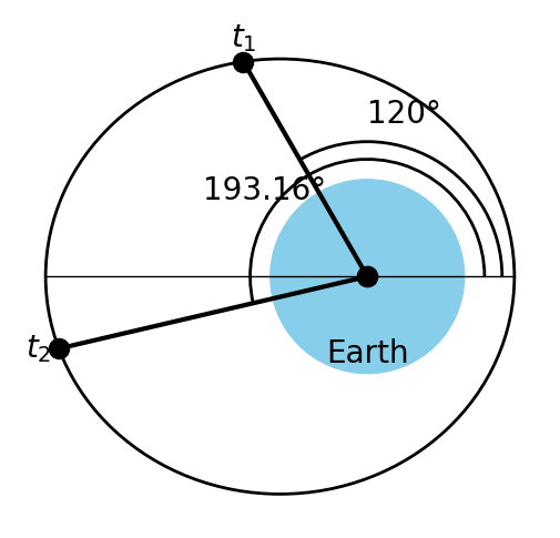
Fig. 52 The orbit in this example showing the two time points, at 120° true anomaly and 3 hours after perigee.