Circular and Elliptical Orbits (\(e < 1\))

As we discussed in the last section, we need to find equations for the mean anomaly and eccentric anomaly. In this section we’ll find three equations that we need:

1. An equation relating the mean anomaly to the time since periapsis:

   \[M_e = \frac{2\pi t}{T} = \frac{\mu^2}{h^3} t \left(1 - e^2\right)^{3/2}\]

2. An equation relating the eccentric anomaly to the true anomaly

   \[\tan\frac{E}{2} = \sqrt{\frac{1 - e}{1 + e}}\tan\frac{\nu}{2}\]

3. An equation relating the mean anomaly to the eccentric anomaly

   \[M_e = E - e \sin{E}\]

With these three equations, we can solve either of the cases of knowing the time since periapsis; or knowing the true anomaly.

For the circle and ellipse, we will follow two methods to derive the appropriate equations:

1. Using a geometric argument to relate swept areas on the orbit and a circumscribing circle

2. Using calculus and trigonometric transformations starting from the orbit equation

These methods result in the same result, but some people may find one easier to follow than the other.

Swept Area Inside the Orbit

Since Kepler’s second law says that equal areas are swept in equal times, the swept area is directly proportional to the elapsed time. Let’s define a variable to capture this idea and call it the Mean Area, \(A_m\):

(185)\[A_m = C t\]

where \(C\) is the constant of proportionality. For an elliptical orbit, the swept area is the elapsed fraction of the orbital period (\(t/T\)) multiplied by the total area of the ellipse (\(\pi a b\)):

We’ll use the example of an ellipse here, but the procedure shown here is similar for a parabola or hyperbola. They just end up with different values for \(C\).

(186)\[A_m = C t = \pi a b \frac{t}{T}\]

where \(a\) and \(b\) are the semimajor and semiminor axes, and \(T\) is the orbital period.

Fig. 49 The swept area \(m_1\)-\(P\)-\(B\) inside the elliptical orbit corresponding to time \(t\) with true anomaly \(\nu\)

This area is shown in Fig. 49 as \(m_1\)-\(P\)-\(B\).

Swept Area Inside a Circumscribing Circle

The next step is find another equation for \(A_m\) so that we can solve for \(t\) in Eq. (186). We already used Kepler’s second law to define Eq. (186), so continuing to work with the ellipse will be kind of a pain.

The circle here is called an circumscribing circle because it is tangent to the ellipse at two points, on both ends of the major axis. These positions are also the periapsis and apoapsis.

Instead, we can work with a circle, where it’s much easier to calculate areas. We are going to transform the ellipse into a circle by stretching it in the vertical direction, ensuring that the circle and ellipse continue to touch at the point \(P\). While the ellipse is stretching, the swept area is also stretching. This process is animated in Fig. 50.

Fig. 50 Transforming the original elliptical orbit into a circumscribing circle by stretching the ellipse in the vertical direction. Note that the point \(B\) translates vertically to point \(Q\).

Notice that the original area \(m_1\)-\(P\)-\(B\) has been transformed to the area \(m_1\)-\(P\)-\(Q\). Our goal now is to find the new area, then scale that area back down to the right size for Eq. (186). To find the area \(m_1\)-\(P\)-\(Q\), we make two observations:

1. The region \(O\)-\(P\)-\(Q\) is a circular sector

2. The region \(O\)-\(m_1\)-\(Q\) is a triangle

These regions are shown on Fig. 51.

Fig. 51 Areas within the circular sector formed by transforming the original ellipse. Note that the original ellipse has been removed from this figure for clarity and only the circumscribing circle is present.

Using these regions, we can find the area \(m_1\)-\(P\)-\(Q\):

(187)\[m_1\text{-}P\text{-}Q = O\text{-}P\text{-}Q - O\text{-}m_1\text{-}Q = \frac{a^2 E}{2} - \frac{a^2 e \sin{E}}{2}\]

where \(a\) is the semimajor axis of the ellipse and the radius of the circle, \(E\) is the included angle in the circular sector, and \(e\) is the eccentricity of the ellipse.

Relating the Two Areas Together

The final step is to scale the area \(m_1\)-\(P\)-\(Q\) back down to the right size and then equate it with \(A_m\). The scaling factor for \(m_1\)-\(P\)-\(Q\) is the ratio of the semi-minor axis, \(b\), to the semi-major axis, \(a\):

\[A_m = \frac{b}{a} \left(m_1\text{-}P\text{-}Q\right) = \frac{abE}{2} - \frac{abe \sin{E}}{2} = \frac{1}{2} a b \left(E - e \sin{E}\right)\]

where we have substituted the result of Eq. (187) and simplified. Finally, substituting Eq. (186):

(188)\[\pi a b \frac{t}{T} = \frac{1}{2}a b \left(E - e \sin{E}\right) \rightarrow 2\pi\frac{t}{T} = E - e \sin{E}\]

In Eq. (188), we can define the left side of the equation as the mean anomaly:

(189)\[M_e = 2\pi\frac{t}{T} = \frac{\mu^2}{h^3} t \left(1 - e^2\right)^{3/2}\]

where \(T\) is the orbital period, \(\mu\) is the specific gravitational constant, \(h\) is the specific angular momentum, and \(e\) is the eccentricity of the orbit. The last equality comes from the definition of the orbital period, Eq. (138).

Substituting Eq. (189) into Eq. (188), we find Kepler’s Equation for an ellipse:

(190)\[M_e = E - e \sin{E}\]

Note

This equation is super important in the field of orbital mechanics, which is why it’s named for Kepler. Make sure to remember this equation!

Now we have two of the three equations we need to solve problems relating elapsed time and true anomaly:

1. Eq. (189) gives us a relationship between \(t\) and \(M_e\)

2. Kepler’s equation, Eq. (190) gives us the relationship between \(M_e\) and \(E\)

The last step is to relate the eccentric anomaly to the true anomaly.

Eccentric Anomaly

The eccentric anomaly, \(E\), is defined as the angle from the \(x\) axis to a point on a circle that circumscribes the orbital ellipse and where the point is located vertically above a point with true anomaly \(\nu\) on the ellipse. This is shown in Fig. 48 and Fig. 52.

Fig. 52 The eccentric anomaly. The blue ellipse is the trajectory of the spacecraft; the green circle is circumscribed around the ellipse. Point \(O\) is the origin, point \(F\) is the focus of the ellipse, point \(S\) is the spacecraft, point \(P\) is the intersection of the apse line and a perpendicular line through \(S\), and point \(Q\) is the intersection of the circle and the perpendicular line through \(S\).

From Fig. 52, we see that the distance \(OP\) is equal to:

(191)\[OP = ae + FP = a \cos E\]

where \(a\) is the semimajor axis of the ellipse, \(e\) is the eccentricity, and the distance \(FP\) is related to the true anomaly:

(192)\[FP = r \cos\nu\]

Combining Eq. (191) and Eq. (192), we find:

(193)\[a\cos E = ae + r\cos\nu\]

Replacing \(r\) with the orbit equation in terms of the semimajor axis and simplifying, we find:

(194)\[\cos E = \frac{e + \cos\nu}{1 + e\cos\nu}\]

or, solving for \(\nu\):

(195)\[\cos\nu = \frac{e - \cos E}{e\cos E - 1}\]

Unfortunately, these equations result in a quadrant ambiguity. We can resolve this by some further trigonometric transformations, which result in the equation:

(196)\[\tan\frac{E}{2} = \sqrt{\frac{1 - e}{1 + e}}\tan\frac{\nu}{2}\]

The inverse tangent function is not multi-valued for a given value of \(\nu\) or \(E\), so this resolves the quadrant ambiguity.

Note

Note: Eq. (196) can be solved in Python with np.arctan() and in Matlab with atan(). It is not necessary to use np.arctan2() or atan2(). Make sure all your arguments are in terms of radians!

Now with Eqs. (190), (196), and (189) we have the three equations we need to solve time since periapsis problems!

Hint

The next section describes an alternate means of deriving these equations from calculus and trigonometric manipulations. I find these derivations interesting, but you may not! Feel free to skip to the examples in the next pages, starting with Example: Elliptical Orbit.

An Alternative Derivation

Now we will pursue the second way to derive Kepler’s equation and the related equations for mean and eccentric anomaly. Recall the orbit equation, Eq. (113), defined in terms of the true anomaly:

\[r = \frac{h^2}{\mu} \frac{1}{1 + e\cos\nu}\]

We now want to relate the true anomaly, \(\nu\), to time. The rate of change of the true anomaly, \(\dot{\nu}\) is equal to the angular velocity of the position vector. This is exactly the azimuthal, also called the perpendicular, component of the velocity:

(197)\[v_{\perp} = r \dot{\nu} = r \frac{d\nu}{dt}\]

The \(v_{\perp}\) term in Eq. (197) makes the equation more complicated than it needs to be, so we’d like to replace it. A more convenient form of Eq. (197) is found by using the specific angular momentum to replace \(v_{\perp}\), since \(h\) is constant:

(198)\[h = r v_{\perp} = r^2\dot{\nu} \Rightarrow \frac{d\nu}{dt} = \frac{h}{r^2}\]

Substituting the orbit equation to eliminate \(r\) and separating variables, we find:

(199)\[\frac{\mu^2}{h^3}dt = \frac{d\nu}{\left(1 + e\cos\nu\right)^2}\]

Since \(\mu\) and \(h\) are constant, the left side can be directly integrated:

(200)\[\frac{\mu^2}{h^3}\int_{t_p}^{t} dt = \int_{0}^{\nu}\frac{d\nu}{\left(1 + e\cos\nu\right)^2}\]

where \(t_p\) is defined as the time since periapsis. Remember that periapsis is when \(\nu = 0\) by convention. Typically we will set \(t_p = 0\), such that:

(201)\[\frac{\mu^2}{h^3}t = \int_{0}^{\nu}\frac{d\nu}{\left(1 + e\cos\nu\right)^2}\]

The integral on the right-hand side of Eq. (201) can be found in standard tables of integrals [GradshteuinRJ07, Zwi03]. There are three forms of the equation, depending on the value of \(e\). In this section, we’ll show the equation for \(e < 1\) and the other equations will be shown in the sections for the parabola and hyperbola.

In [GradshteuinRJ07] (available here), the appropriate integrals are found on pages 172 and 173, No. 2.554-3 and related integrals for Eqs. (202) and (223). In [Zwi03] (available here), the appropriate integrals are found on pages 433 and 434, No. 354 and 324 for Eqs. (202) and (223). I couldn’t find the form for (217) in those references. Note that \(a = 1\) and \(b = e\) to relate the reference equations to Eq. (201).

(202)\[\int\frac{d\nu}{\left(1 + e\cos \nu\right)^2} = \frac{1}{\left(1 - e^2\right)^{3/2}}\left[2\tan^{-1}\left(\sqrt{\frac{1 - e}{1 + e}}\tan\frac{\nu}{2}\right)-\frac{e\sqrt{1 - e^2}\sin \nu}{1 + e \cos \nu}\right]\]

In Eq. (202), \(e < 1\), so it will apply for circular and elliptical orbits.

When Eq. (201) is combined with Eq. (202) we have a relationship where time is related to the true anomaly.

For circular and elliptical orbits, combining Eq. (201) and Eq. (202) results in:

(203)\[\frac{\mu}{h^3}t = \frac{1}{\left(1 - e^2\right)^{3/2}}\left[2\tan^{-1}\left(\sqrt{\frac{1 - e}{1 + e}}\tan\frac{\nu}{2}\right)-\frac{e\sqrt{1 - e^2}\sin \nu}{1 + e \cos \nu}\right]\]

Mean Anomaly

We define the term in the square brackets in Eq. (203) to be the mean anomaly, \(M_e\), where the subscript \(e\) indicates that this is for the ellipse. We will have different equations for the parabola and hyperbola.

(204)\[M_e = \left[2\tan^{-1}\left(\sqrt{\frac{1 - e}{1 + e}}\tan\frac{\nu}{2}\right)-\frac{e\sqrt{1 - e^2}\sin \nu}{1 + e \cos \nu}\right]\]

The mean anomaly is a monotonically increasing function of the true anomaly, as shown in Fig. 53. This is good because it means that \(M_e\) can be used in place of \(\nu\) for all four quadrants on the \(x\)-\(y\) plane. If \(M_e\) had a peak, we would have to be concerned about which quadrant we were in.

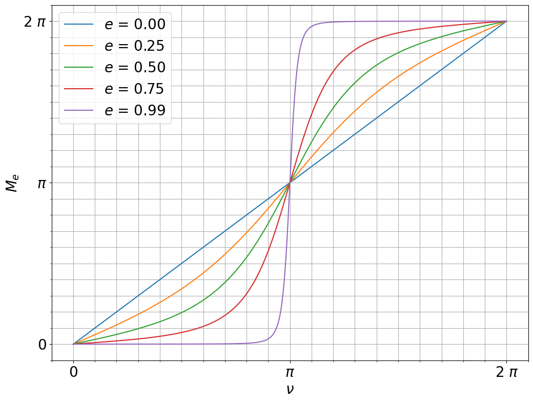
Fig. 53 Mean anomaly as a function of true anomaly for a range of eccentricities. Note that \(e < 1\).

Notice that when \(e = 0\) (a circular orbit), the mean anomaly and true anomaly are equal.

Plugging Eq. (204) into Eq. (203) and solving for \(M_e\), we find:

(205)\[M_e = \frac{\mu^2}{h^3} t \left(1 - e^2\right)^{3/2}\]

If we know the period of the orbit, we can simplify the equation for the mean anomaly:

(206)\[M_e = \frac{2\pi}{T}t\]

For a circle, the mean anomaly equals the true anomaly:

(207)\[\nu_{\text{circle}} = \frac{2\pi}{T} t\]

Further solution is not needed if the orbit is circular. Now we have the relationship between mean anomaly and time that we need for solution of these problems. Note that Eq. (189) and Eqs. (205) and (206) are exactly identical.

The procedure to find the eccentric anomaly is the same as in the previous section, so we can move on to deriving Kepler’s equation.

Kepler’s Equation

Some further trigonometry with Eq. (194), Eq. (196), and Eq. (203) yields Kepler’s Equation:

\[M_e = E - e \sin E\]

This gives the relationship between mean anomaly and eccentric anomaly. The value of \(M_e\) monotonically increases as a function of \(E\), as shown in Fig. 54 for several values of \(e\).

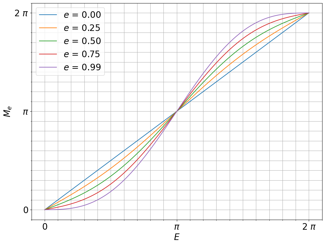
Fig. 54 The mean anomaly as a function of eccentric anomaly for several values of the eccentricity. Note that \(e < 1\).

Solution Procedures

Now we have all the pieces we need to apply the solution procedures discussed in the introductory section.

Given True Anomaly, Find Time Since Periapsis

Given a value of the true anomaly \(\nu\), the eccentric anomaly \(E\) can be calculated from Eq. (196). Then, Kepler’s Equation can be solved to find \(M_e\), and the time since periapsis is found by:

(208)\[t = \frac{M_e}{2\pi} T\]

Given Time Since Periapsis, Find True Anomaly

If, on the other hand, we are given the time since periapsis and want to find the true anomaly, we must first solve Eq. (206) for \(M_e\). Then we need to solve Kepler’s equation for \(E\). Unfortunately, this equation is transcendental in \(E\), so it cannot be solved analytically. There are several methods to solve Kepler’s equation, depending on the level of accuracy required and the access to computational tools.

Once \(E\) is determined, Eq. (196) can be solved for \(\nu\).

Newton’s Method to Solve Kepler’s Equation

For Newton’s method, we seek the roots of a function, \(f(E) = 0\). In this case, we can rearrange Kepler’s equation as:

(209)\[f(E) = E - e\sin E - M_e\]

It is also convenient to supply the derivative, when it is available, since this improves the convergence rate of the algorithm. The derivative is:

(210)\[\frac{d f(E)}{d E} = f'(E) = 1 - e\cos E\]

These equations can be provided to standard computational solvers for root finding algorithms.

Infinite Series Solutions of Kepler’s Equation

Although there are no analytical solutions for Kepler’s equation, several people have developed infinite series solutions. The first was developed by Lagrange:

(211)\[E = M_e + \sum_{n = 1}^{\infty}a_n e^n\]

where the coefficients \(a_n\) are given by:

(212)\[a_n = \frac{1}{2^{n - 1}} \sum_{k=0}^{\mathrm{floor}(n/2)}(-1)^k\frac{1}{\left(n - k\right)!k!}\left(n - 2k\right)^{n - 1}\sin\left[\left(n - 2k\right)M_e\right]\]

and where \(\mathrm{floor}(x)\) means to take the next lowest integer relative to \(x\).

Note: Sacchetti [Sac20] states that Italian astronomer Francesco Carlini was the first to prove the existence of the convergence limit for the Lagrange series five years before Laplace completed his work. DRAMA!

This infinite series converges for \(e < 0.6627434193\), a limit that was proven by Laplace, and is therefore typically called the Laplace limit. For larger values of \(e\), the series diverges.

Another infinite series was developed by Bessel, which converges for all \(e < 1\):

(213)\[E = M_e + \sum_{n=1}^{\infty}\frac{2}{n} J_n(ne)\sin n M_e\]

where \(J_n\) are the Bessel functions of the first kind, defined by their own infinite series:

(214)\[J_n(x) = \sum_{k=0}^{\infty}\frac{\left(-1\right)^k}{k!\left(n + k\right)!}\left(\frac{x}{2}\right)^{n+ k}\]

There are other feasible series solutions to Kepler’s equation, some of which are discussed by Colwell [Col92].