The Orbit Equation

The Orbit Equation#

Now, we’ll return to the equation of relative motion, Eq. (33), repeated here for reference:

\ddot{r} = - (\frac{μ}{r^{3}}) r

Our goal is to be able to integrate this equation to find a scalar equation. An analytical equation will be more accurate than the numerical techniques we used earlier, and a scalar equation is easier to work with than a vector one.

We start by taking the cross product of this equation with the angular momentum, $h$ :

(110)#

\ddot{r} \times h = - (\frac{μ}{r^{3}}) r \times h

To make this easy to integrate, we want both sides to be $d / d t (\dots)$ . Let’s try to replace the left-hand side of the equation. Since $\ddot{r} = d / d t (\dot{r})$ , lets try to pull a $d / d t$ out. By the product rule of differentiation, we find:

(111)#

\frac{d}{d t} (\dot{r} \times h) = \ddot{r} \times h + \dot{r} \times \dot{h}

But the angular momentum is constant, so its derivative $\dot{h} = 0$ and the second term in Eq. (111) is zero. Therefore:

\frac{d}{d t} (\dot{r} \times h) = \ddot{r} \times h = - (\frac{μ}{r^{3}}) r \times h

So, the left-hand side of the formula is in terms of $d / d t (\dots)$ . Let’s get the right-hand side into the same form so we can simplify. After a bunch of algebra, we find:

- \frac{μ}{r^{3}} r \times h = μ \frac{d}{d t} (\frac{r}{r})

Substituting everything together, we find:

\frac{d}{d t} (\dot{r} \times h) = \frac{d}{d t} (μ \frac{r}{r})

Rearranging:

\frac{d}{d t} (\dot{r} \times h - μ \frac{r}{r}) = 0

This equation can be integrated to find:

\dot{r} \times h - μ \frac{r}{r} = B

where $B$ is called the Laplace vector and is the constant of integration. The Laplace vector has the same dimensions as $μ$ , so we can transform it into a dimensionless number by dividing the equation by $μ$ :

(112)#

\frac{r}{r} + e = \frac{\dot{r} \times h}{μ}

where $e = B / μ$ and is called the eccentricity vector. Since $B$ lies in the orbital plane, $e$ also lies in the orbital plane. The line along $e$ is called the apse line. These coordinates are shown in Fig. 30.

../_images/apse-line.svg — Fig. 30 The eccentricity vector lies in the plane of the orbit, starting at the occupied focus and pointing towards the point of closest approach. A line through this vector is the apse line. The true anomaly is the angle from the apse line to the current position vector from $m_{1}$ to $m_{2}$ .#

We now want to transform Eq. (112) to be in terms of $r$ and $ν$ , which is called the true anomaly, defined as the angle from the apse line to the $m_{2}$ . This will result in a scalar equation, which is easier to work with than the vector equation.

To obtain a scalar equation, we take the dot product of Eq. (112) with $r$ . After some algebra, we end up at:

(113)#

r = \frac{h^{2}}{μ} \frac{1}{1 + e \cos ν}

where $e = ‖ e ‖$ is called the eccentricity. Eq. (113) is called the orbit equation and it defines the path of $m_{2}$ around $m_{1}$ , relative to $m_{1}$ . In this equation, $h$ , $e$ , and $μ$ are all constant. Since $e$ is the magnitude of $e$ , it is strictly positive, $e \geq 0$ .

Important

Put a big star next to Eq. (113). We are going to use it for the rest of the course!

The orbit equation describes conic sections, meaning that all orbits are one of four types, as shown in Fig. 31. The particular type of orbit is determined by the magnitude of the eccentricity:

Circles: $e = 0$
Ellipses: $0 < e < 1$
Parabolas: $e = 1$
Hyperbolas $e > 1$

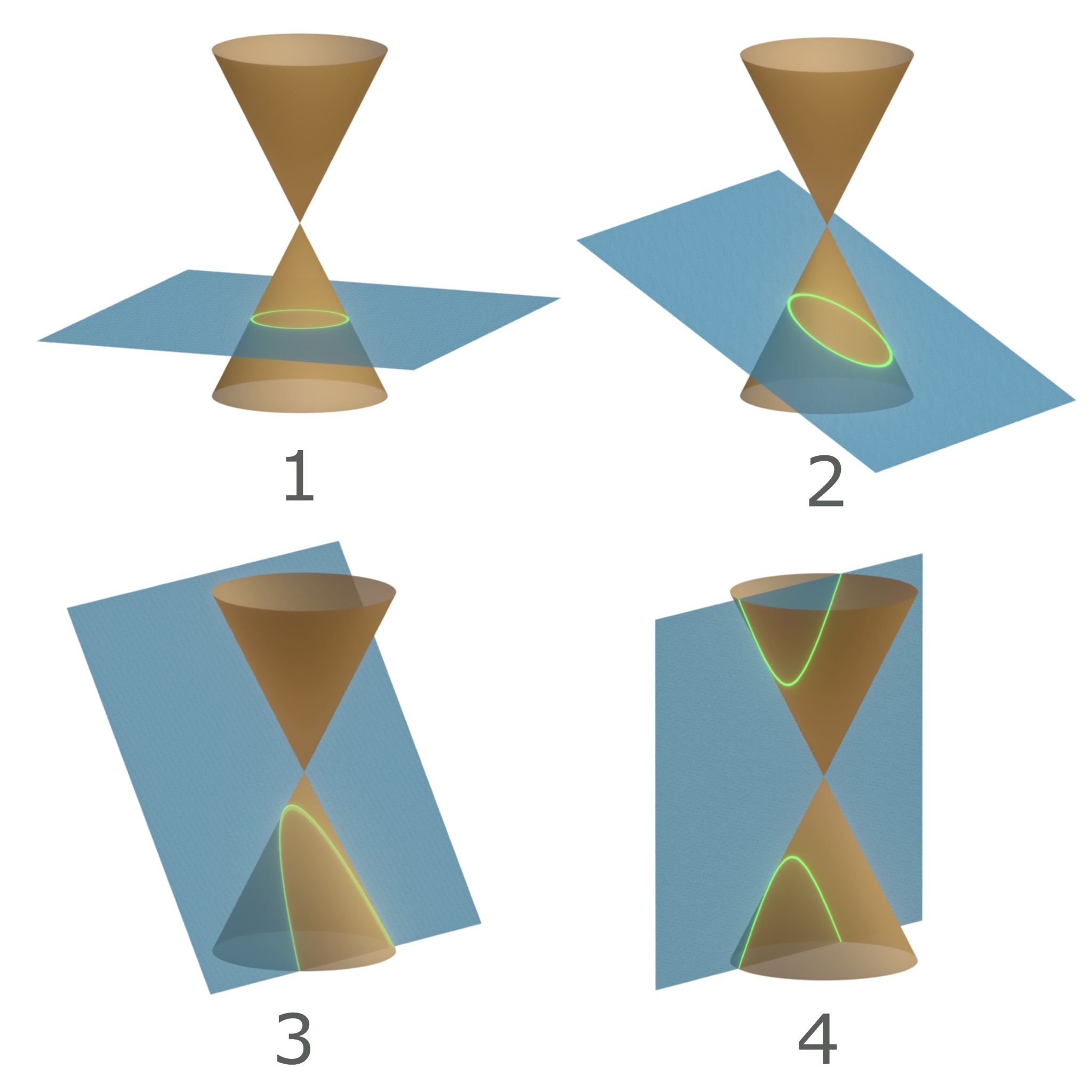
../_images/TypesOfConicSections.jpg — Fig. 31 The 4 types of conic section: 1. Circle; 2. Ellipse; 3. Parabola; 4. Hyperbola. JensVyff, CC BY-SA 4.0, via Wikimedia Commons#

We are going to handle each of these in turn in a few sections. In the meantime, we are going to do a little bit of work directly with the orbit equation.