Example: Plotting Lagrange Points

In this example, we will plot the Lagrange points for the system as a function of \(\pi_2\).

In the nondimensional coordinates, we know that \(L_4\) and \(L_5\) have analytical solutions from Eq. (83) and repeated here for reference:

\[\begin{split}\begin{aligned} &L_4: & x^* &= \frac{1}{2} - \pi_2 & y^* &= \frac{\sqrt{3}}{2} \\ &L_5: & x^* &= \frac{1}{2} - \pi_2 & y^* &= -\frac{\sqrt{3}}{2} \end{aligned}\end{split}\]

However, the collinear Lagrange points do not have an analytical solution, and must be approximated numerically. To do so, we will use scipy.optimize.newton() in Python and fzero in Matlab.

The formula for the nondimensional position of the collinear Lagrange points is given by Eq. (86), repeated here for reference:

\[0 = x^* - \frac{1 - \pi_2}{\left\lvert x^* + \pi_2\right\rvert ^3}\left(x^* + \pi_2\right) - \frac{\pi_2}{\left\lvert x^* - 1 + \pi_2\right\rvert ^3}\left(x^* - 1 + \pi_2\right)\]

Here, we have a function \(f(x^*, \pi_2)\), which for a given value of \(\pi_2\) has three roots for \(x^*\), one for each of the collinear Lagrange points. From Fig. 15, we can determine the range of \(x^*\) values associated with each point.

• \(L_2\): \(1 < x^* < 1.25\)

• \(L_1\): \(-1 < x^* < 1\)

• \(L_3\): \(-1.25 < x^* < -1\)

Both scipy.optimize.newton and fzero depend on having a good initial guess to get to the right Lagrange point. My suggestion is to use the following initial guess range for both functions, depending on which Lagrange point you’re looking for:

• \(L_2\):

  • Python (scipy.optimize.newton): x0=1

  • MATLAB (fzero): [1, 1.5]

• \(L_1\):

  • Python (scipy.optimize.newton): x0=0

  • MATLAB (fzero): Either [0, -0.5] or [0, 0.5] depending on the value of \(\pi_2\)

• \(L_3\):

  • Python (scipy.optimize.newton): x0=-1

  • MATLAB (fzero): [-1, -1.5]

For some reason, the fzero() in MATLAB seems much more sensitive to the initial guess value, and if you only provide a single value for the initial guess, it chooses a positive value as the second part of the interval. Thus, if the root is below your initial guess the MATLAB solver will not be able to find it.

Python

First, we will demonstrate the Python solver. Like for the solve_ivp function, we need to define a function that returns a value given the single input xstar. Python is flexible enough to allow us to define pi_2 as another parameter.

# %matplotlib notebook
import matplotlib.path as mpath
import matplotlib.pyplot as plt
import numpy as np
from scipy.optimize import newton

# This code defines a nice shape for the center of mass of the system.
circle = mpath.Path.unit_circle()
wedge_1 = mpath.Path.wedge(90, 180)
wedge_2 = mpath.Path.wedge(270, 0)

verts = np.concatenate(
    [circle.vertices, wedge_1.vertices[::-1, ...], wedge_2.vertices[::-1, ...]]
)
codes = np.concatenate([circle.codes, wedge_1.codes, wedge_2.codes])
center_of_mass = mpath.Path(verts, codes)

# These masses represent the Earth-Moon system
m_1 = 5.974e24  # kg
m_2 = 7.348e22  # kg
pi_2 = m_2 / (m_1 + m_2)

# These give us the coordinates of the orbits of m_2 and m_1
x_2 = (1 - pi_2) * np.cos(np.linspace(0, np.pi, 100))
y_2 = (1 - pi_2) * np.sin(np.linspace(0, np.pi, 100))
x_1 = (-pi_2) * np.cos(np.linspace(0, np.pi, 100))
y_1 = (-pi_2) * np.sin(np.linspace(0, np.pi, 100))

def collinear_lagrange(xstar, pi_2):
    """Calculate the resultant of the collinear Lagrange point equation.

    This is a function f(xstar, pi_2), where xstar is the nondimensional x coordinate
    and pi_2 is the nondimensional mass ratio. The function should be passed to
    scipy.optimize.newton (or another Newton solver) to find a value for xstar
    that satsifies the equation, for a given value of pi_2.

    The solver will try different values of xstar until the return value is equal to
    zero.
    """
    first_term = xstar
    second_term = (1 - pi_2) / np.abs(xstar + pi_2) ** 3 * (xstar + pi_2)
    third_term = pi_2 / np.abs(xstar - 1 + pi_2) ** 3 * (xstar - 1 + pi_2)
    return first_term - second_term - third_term

Then we need to pass this to the Newton solver. The function signature is:

newton(func, x0, args)

where func is the function to be solved, x0 is the initial guess, and args is a tuple of additional arguments to pass to func.

L_2 = newton(func=collinear_lagrange, x0=1, args=(pi_2,))
L_1 = newton(func=collinear_lagrange, x0=0, args=(pi_2,))
L_3 = newton(func=collinear_lagrange, x0=-1, args=(pi_2,))
print(f"{L_1=}, {L_2=}, {L_3=}")

L_1=0.8369154703225321, L_2=1.1556818961296604, L_3=-1.0050626166357435

Remember, these are in nondimensional coordinates. We can then plot the Lagrange points relative to \(m_1\) and \(m_2\) in the rotating frame of reference.

fig, ax = plt.subplots(figsize=(5, 5), dpi=96)
ax.set_xlabel("$x^*$")
ax.set_ylabel("$y^*$")

# Plot the orbits
ax.axhline(0, color="k")
ax.plot(np.hstack((x_2, x_2[::-1])), np.hstack((y_2, -y_2[::-1])))
ax.plot(np.hstack((x_1, x_1[::-1])), np.hstack((y_1, -y_1[::-1])))
ax.plot(
    [-pi_2, 0.5 - pi_2, 1 - pi_2, 0.5 - pi_2, -pi_2],
    [0, np.sqrt(3) / 2, 0, -np.sqrt(3) / 2, 0],
    "k",
    ls="--",
    lw=1,
)

# Plot the Lagrange Points and masses
ax.plot(L_1, 0, "rv", label="$L_1$")
ax.plot(L_2, 0, "r^", label="$L_2$")
ax.plot(L_3, 0, "rp", label="$L_3$")
ax.plot(0.5 - pi_2, np.sqrt(3) / 2, "rX", label="$L_4$")
ax.plot(0.5 - pi_2, -np.sqrt(3) / 2, "rs", label="$L_5$")
ax.plot(0, 0, "k", marker=center_of_mass, markersize=10)
ax.plot(-pi_2, 0, "bo", label="$m_1$")
ax.plot(1 - pi_2, 0, "go", label="$m_2$")
ax.legend()
ax.set_aspect("equal")

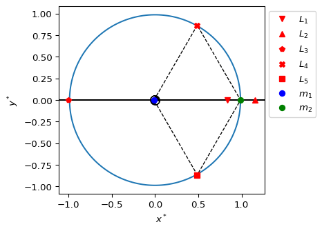
Fig. 20 The location of the Lagrange points in the Earth-Moon system, shown in non-dimensional coordinates.

Matlab

In MATLAB, we are using fzero as the solver. The code below produces the same output as the Python code above.

function lagrange_points_example
    % These masses represent the Earth-Moon system
    m1 = 5.974E24; % kg
    m2 = 7.348E22; % kg
    pi2 = m2/(m1 + m2);

    function y = collinear_lagrange(xstar)
        firstterm = xstar;
        secondterm = (1 - pi2) ./ abs(xstar + pi2).^3 .* (xstar + pi2);
        thirdterm = pi2 ./ abs(xstar - 1 + pi2).^3 .* (xstar - 1 + pi2);
        y = firstterm - secondterm - thirdterm;
    end
    options = optimset('Display','iter');
    L_2 = fzero(@collinear_lagrange,[1, 1.5],options);
    L_1 = fzero(@collinear_lagrange,[0.01, 0.97],options);
    L_3 = fzero(@collinear_lagrange,[-1, -1.5],options);
    fprintf('L_1=%f, L_2=%f, L_3=%f\n', L_1, L_2, L_3)

    function output
        figure()
        title('The Lagrange Points in the Earth-Moon System')
        hold on
        ylim([-1.2,1.2])
        xlim([-1.2,1.2])
        axis square
        xlabel('x^*')
        ylabel('y^*')
        plot(-pi2,0,'bo','MarkerFaceColor','b')
        plot(1-pi2,0,'go','MarkerFaceColor','g')
        plot(L_1,0,'rv','MarkerFaceColor','r')
        plot(L_2,0,'r^','MarkerFaceColor','r')
        plot(L_3,0,'rp','MarkerFaceColor','r')
        plot(0.5-pi2,sqrt(3)/2,'rX','MarkerFaceColor','r')
        plot(0.5-pi2,-sqrt(3)/2,'rs','MarkerFaceColor','r')
        plot([-pi2,0.5-pi2,1-pi2,0.5-pi2,-pi2], [0,sqrt(3)/2,0,-sqrt(3)/2,0], '--k')
        yline(0,'k')
        coords = linspace(0,pi,100);
        plot((1-pi2).*cos(coords),(1-pi2).*sin(coords))
        hold all
        plot((1-pi2).*cos(coords),-(1-pi2).*sin(coords))
        legend('$m_1$','$m_2$', '$L_1$', '$L_2$', '$L_3$', '$L_4$', '$L_5$','Interpreter','latex')
    end
    output
end

Notice that to find \(L_1\) in Matlab, we had to use the initial guess range from 0.01 to 0.97. Matlab is more sensitive to the initial guess, so you need to make sure that the root is within the initial guess you choose. The collinear_lagrange function is discontinuous around 0 and 1.0, so you need to choose your limits carefully.

It may help to plot the function for a given problem. To do so, within the script, add the line fplot(@collinear_lagrange) to show a plot of the function.