Hyperbolic Trajectories (\(e > 1\))

For the hyperbola, combining Eq. (189) and Eq. (192) results in:

(219)\[M_h = \frac{e\sqrt{e^2 - 1}\sin\nu}{1 + e\cos\nu} - \ln\left[\frac{\sqrt{e + 1} + \sqrt{e - 1}\tan\frac{\nu}{2}}{\sqrt{e + 1} - \sqrt{e - 1}\tan\frac{\nu}{2}}\right]\]

where

(220)\[M_h = \frac{\mu^2}{h^3} t \left(e^2 - 1\right)^{3/2}\]

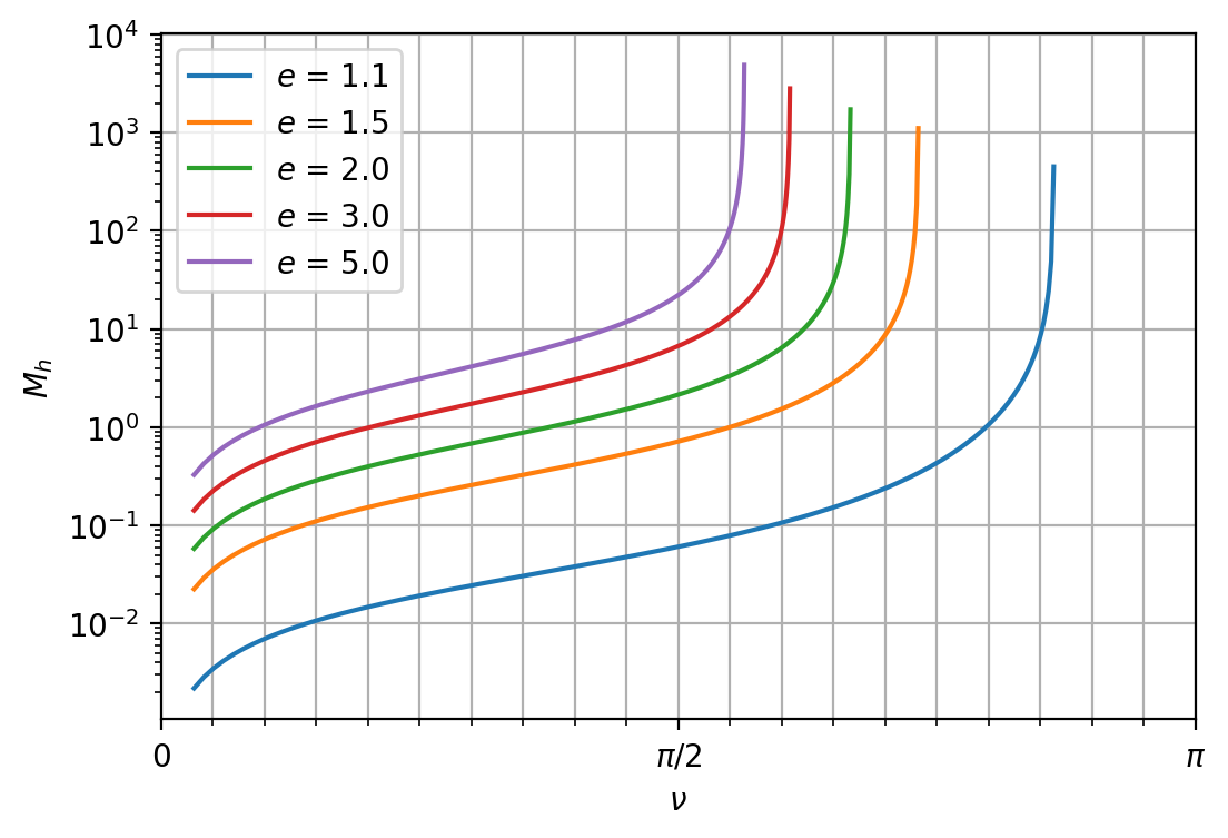
The hyperbolic mean anomaly, like the elliptical mean anomaly, is a monotonic function of the true anomaly, as shown in Fig. 55.

Fig. 55 The hyperbolic mean anomaly as a function of true anomaly. Note that the \(y\)-scale is a log scale.

Notice that \(\nu\) cannot exceed \(\nu_{\infty} = \cos^{-1}(-1 / e)\).

Hyperbolic Eccentric Anomaly

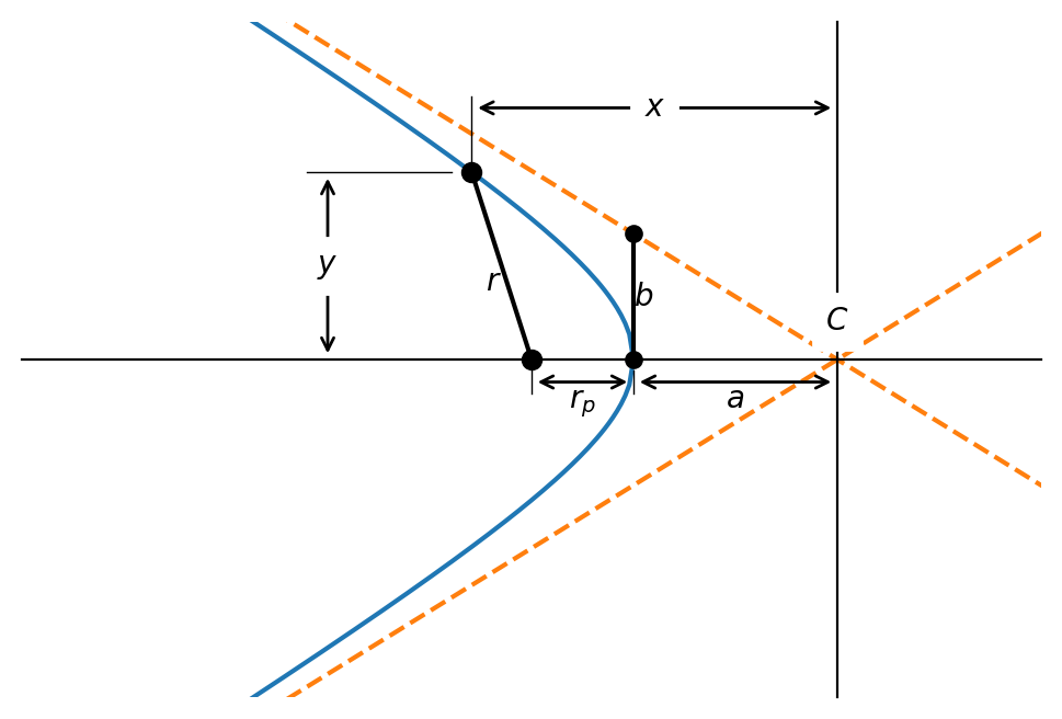
Similar to the ellipse, we will define an auxiliary angle \(F\) to simplify the equations. \(F\) is defined with reference to the hyperbola in Fig. 56.

Fig. 56 A hyperbolic trajectory with definitions for distances used in the derivation of Kepler’s law for hyperbolic.

The ratio \(y/b\) is the definition of the hyperbolic sine of the angle \(F\):

(221)\[\sinh F = \frac{y}{b}\]

Then, using the hyperbolic trigonometric identity:

(222)\[\cosh^2 c - \sinh^2 c = 1\]

we also define

(223)\[\cosh F = \frac{x}{a}\]

Note

The hyperbolic angle \(F\) is weird. The reason we don’t draw it on the figure is because hyperbolic angles aren’t angles per se. Instead, they can be interpreted as half the area between the \(x\)-axis and a line drawn from the origin to the point of interest, bounded by the hyperbola. I think. At least, that’s my best interpretation from what I’ve been able to read. YMMV.

Another way of thinking about this is by analogy to a circle. For a circle, we can draw any two lines from the center of the circle to the perimeter. These two lines will have an angle \(\phi\) between them, and the area between them will be:

(224)\[A_{\text{circular sector}} = \frac{r^2 \phi}{2}\]

Fig. 57 The highlighted area is a circular sector. Modified from Wikimedia.

If the circle is a unit circle (\(r = 1\)), then the area of the sector will be equal to the angle divided by two. Turned around, the angle is equal to twice the area:

(225)\[\phi = \frac{2A}{1^2}\]

Similarly, the hyperbolic angle is defined on the unit hyperbola as twice the area between two lines that start at the origin and touch the hyperbola, called a hyperbolic sector.

Fig. 58 The area of the hyperbolic sector is half the hyperbolic angle. Hyperbolic_functions.svg: The original uploader was Marco Polo at English Wikipedia.derivative work: Jeandavid54, Public domain, via Wikimedia Commons

However, the circular angle between the \(x\)-axis and the ray from the origin is not the same as the hyperbolic angle.

You can read more about hyperbolic angles on Brilliant and on Wikipedia.

We can relate \(F\) to the true anomaly \(\nu\) by plugging in \(y = r\sin\nu\), and the orbit equation for \(r\). We also note that \(b = a\sqrt{e^2 - 1}\). Then:

(226)\[F = \sinh^{-1}\left(\frac{\sin\nu\sqrt{e^2 - 1}}{1 + e\cos\nu}\right) = \ln\left(\frac{\sin\nu\sqrt{e^2 - 1} + \cos\nu + e}{1 + e\cos\nu}\right)\]

After some more trigonometry and algebra, we find:

(227)\[F= \ln\left[\frac{\sqrt{e + 1} + \sqrt{e - 1}\tan\frac{\nu}{2}}{\sqrt{e + 1} - \sqrt{e - 1}\tan\frac{\nu}{2}}\right]\]

And, with a little more algebra and trigonometry, we find an equation for \(F\) in terms of \(\nu\) more directly, analogous to the ellipse:

(228)\[\tanh\frac{F}{2} = \sqrt{\frac{e - 1}{e + 1}}\tan\frac{\nu}{2}\]

Kepler’s Equation for the Hyperbola

Substituting this back into Eq. (219), we find Kepler’s equation for the hyperbola:

(229)\[M_h = e\sinh F - F\]

As with the ellipse, Kepler’s equation can be solved easily if \(F\) is known. However, if time is the known quantity, then Kepler’s equation is transcendental and must be solved numerically. The form of the equation for the Newton solver is \(f(F) = 0\), or:

(230)\[f(F) = 0 = e\sinh F - F - M_h\]

To aid in the numerical solution, the derivative of Kepler’s equation for the hyperbola is:

(231)\[f'(F) = e \cosh F - 1\]

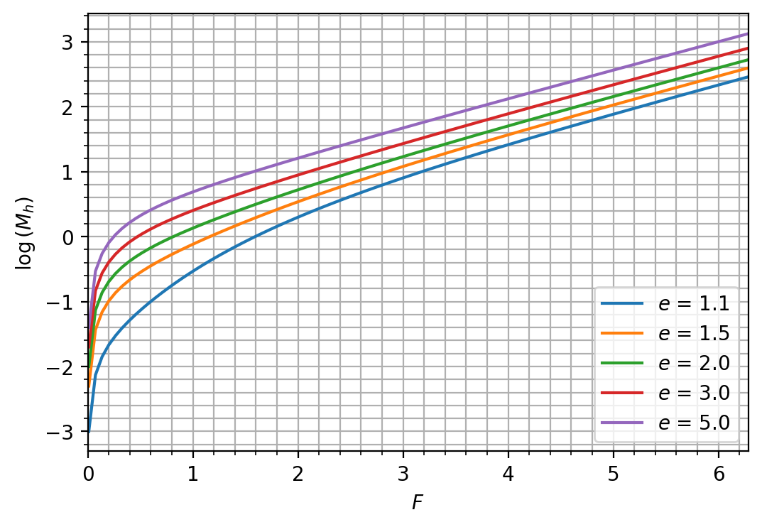
In addition, we can estimate an initial value for the guess of \(F\) from Fig. 59, with a known \(M_h\) value.

Fig. 59 The hyperbolic mean anomaly as a function of the eccentric anomaly

Note that the \(y\)-axis plots the log base 10 of \(M_h\). To use the graph, take the log base 10 of whatever value you calculate for \(M_h\) and find that on the graph. For example, assume that \(M_h =\) 40.69 rad and \(e =\) 2.5. Then,

\[\log_{10}(40.69) = 1.6\]

From Fig. 59, we estimate that \(F =\) 4, and we can use this as the initial guess for a Newton solver.