Example: CR3BP Equations of Motion

Equation (71) shows the three nondimensional scalar equations of motion for the CR3BP, repeated here for reference:

\[\begin{split}\begin{aligned} \ddot{x}^* - 2\dot{y}^* - x^* &= -\frac{1 - \pi_2}{\sigma^3}\left(x^* + \pi_2\right) - \frac{\pi_2}{\psi^3}\left(x^* - 1 + \pi_2\right) \\ \ddot{y}^* + 2\dot{x}^* - y^* &= -\frac{1 - \pi_2}{\sigma^3} y^* - \frac{\pi_2}{\psi^3}y^* \\ \ddot{z}^* &= -\frac{1 - \pi_2}{\sigma^3}z^* - \frac{\pi_2}{\psi^3}z^* \end{aligned}\end{split}\]

In this example, we will solve this system of equations numerically for the position of the tertiary mass \(m\) as a function of time in the rotating frame of reference. The state vector in this problem is the same as in the relative motion case. There are six elements of the state vector:

(92)\[Y = \left[x^*\ y^*\ z^*\ \dot{x}^*\ \dot{y}^*\ \dot{z}^*\right]^T\]

To put Eq. (71) into a form that we can solve, we need to solve for the acceleration components:

\[\begin{split}\begin{aligned} \ddot{x}^* &= 2\dot{y}^* + x^* - \frac{1 - \pi_2}{\sigma^3} \left(x^* + \pi_2\right) - \frac{\pi_2}{\psi^3}\left(x^* - 1 + \pi_2\right) \\ \ddot{y}^* &= -2\dot{x}^* + y^* - \frac{1 - \pi_2}{\sigma^3} y^* - \frac{\pi_2}{\psi^3}y^* \\ \ddot{z}^* &= -\frac{1 - \pi_2}{\sigma^3}z^* - \frac{\pi_2}{\psi^3}z^* \end{aligned}\end{split}\]

We need to provide \(\pi_2\), the mass ratio, as the parameter of the system, along with the initial position and velocity. Let’s solve this system of equations numerically to find the position of \(m\) as a function of non-dimensional time in the rotating frame of reference. First, we import the appropriate libraries:

import matplotlib.pyplot as plt
import numpy as np
from scipy.integrate import solve_ivp

# These masses represent the Earth-Moon system
m_1 = 5.974e24  # kg
m_2 = 7.348e22  # kg
pi_2 = m_2 / (m_1 + m_2)

The system of equations is very sensitive to the initial conditions that we pick. In this case, we are choosing the initial position at the \(x^*\) position of the secondary mass, offset slightly in the \(y^*\) axis. The initial velocity is directed along the positive \(y^*\) axis and the negative \(x^*\) axis.

x_0 = 1 - pi_2
y_0 = 0.0455
z_0 = 0
vx_0 = -0.5
vy_0 = 0.5
vz_0 = 0

# Then stack everything together into the state vector
r_0 = np.array((x_0, y_0, z_0))
v_0 = np.array((vx_0, vy_0, vz_0))
Y_0 = np.hstack((r_0, v_0))

Now we need to define the function that solves the non-dimensional equations of motion, much like the function in the relative motion problem.

def nondim_cr3bp(t, Y):
    """Solve the CR3BP in nondimensional coordinates.

    The state vector is Y, with the first three components as the
    position of $m$, and the second three components its velocity.

    The solution is parameterized on $\\pi_2$, the mass ratio.
    """
    # Get the position and velocity from the solution vector
    x, y, z = Y[:3]
    xdot, ydot, zdot = Y[3:]

    # Define the derivative vector
    Ydot = np.zeros_like(Y)
    Ydot[:3] = Y[3:]

    sigma = np.sqrt(np.sum(np.square([x + pi_2, y, z])))
    psi = np.sqrt(np.sum(np.square([x - 1 + pi_2, y, z])))
    Ydot[3] = (
        2 * ydot
        + x
        - (1 - pi_2) * (x + pi_2) / sigma**3
        - pi_2 * (x - 1 + pi_2) / psi**3
    )
    Ydot[4] = -2 * xdot + y - (1 - pi_2) * y / sigma**3 - pi_2 * y / psi**3
    Ydot[5] = -(1 - pi_2) / sigma**3 * z - pi_2 / psi**3 * z
    return Ydot

Now we can solve the problem with solve_ivp(). We choose an end time of 25 non-dimensional units, pretty much arbitrarily to see what we can get.

t_0 = 0  # nondimensional time
t_f = 20  # nondimensional time
t_points = np.linspace(t_0, t_f, 1000)
sol = solve_ivp(nondim_cr3bp, [t_0, t_f], Y_0, t_eval=t_points)

Y = sol.y.T
r = Y[:, :3]  # nondimensional distance
v = Y[:, 3:]  # nondimensional velocity

Finally, to plot the trajectory, we will define some values for the circular orbit of \(m_2\) around the barycenter and then plot the trajectory of \(m\) in red.

x_2 = (1 - pi_2) * np.cos(np.linspace(0, np.pi, 100))
y_2 = (1 - pi_2) * np.sin(np.linspace(0, np.pi, 100))
fig, ax = plt.subplots(figsize=(5, 5), dpi=96)

# Plot the orbits
ax.plot(r[:, 0], r[:, 1], "r", label="Trajectory")
ax.axhline(0, color="k")
ax.plot(np.hstack((x_2, x_2[::-1])), np.hstack((y_2, -y_2[::-1])))
ax.plot(-pi_2, 0, "bo", label="$m_1$")
ax.plot(1 - pi_2, 0, "go", label="$m_2$")
ax.plot(x_0, y_0, "ro")
ax.set_aspect("equal")

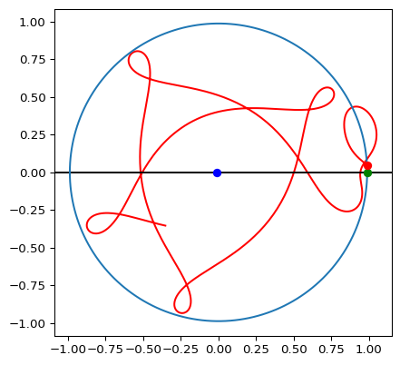
Fig. 22 The trajectory of \(m\) in the rotating frame of reference, in non-dimensional coordinates.

As shown in Fig. 22, we can get some very interesting behavior of \(m\) in the rotating frame of reference. The behavior of \(m\) depends very strongly on the initial conditions that we set.

Calculating the Jacobi Constant

In the nondimensional coordinates, the Jacobi constant is given by Eq. (90), repeated here for reference:

\[J = \frac{1}{2} \left(v^*\right)^2 - \frac{1 - \pi_2}{\sigma} - \frac{\pi_2}{\psi} - \frac{1}{2}\left[\left(1 - \pi_2\right)\sigma^2 + \pi_2 \psi^2\right]\]

This value should be constant over the entire trajectory of the tertiary mass.

speed_sq = np.sum(np.square(v), axis=1)

r[:, 0] += pi_2
sigma = np.sqrt(np.sum(np.square(r), axis=1))
r[:, 0] -= 1.0
psi = np.sqrt(np.sum(np.square(r), axis=1))
r[:, 0] = r[:, 0] + 1.0 - pi_2

J = (
    0.5 * speed_sq
    - (1 - pi_2) / sigma
    - pi_2 / psi
    - 0.5 * ((1 - pi_2) * sigma**2 + pi_2 * psi**2)
)

Now that we have calculated \(J\) as a function of time, let’s plot it! Hopefully it’s constant…

fig, ax = plt.subplots(figsize=(8, 6), dpi=96)
ax.plot(sol.t, J, label="Jacobi Constant")
ax.axhline(J[0], color="C1", label="Initial Jacobi Constant")
ax.legend(loc="center left")
ax.set_xlabel("$\\tau$")
ax.set_ylabel("$J$")

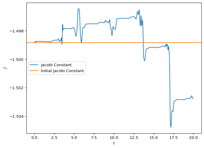
Fig. 23 The Jacobi constant, \(J\), as a function of non-dimensional time. The horizontal line is the initial Jacobi constant.

Oh dear. Fig. 23 shows that the Jacobi constant varies by about 0.02 over the trajectory. Keep in mind that a change of \(J\) on the order of \(10^{-2}\) is the difference from the \(L_1\) and \(L_2\) points being accessible in the Earth-Moon system. So a change of \(2\times 10^{-2}\) is quite large on that scale.

Tighten the Integrator Tolerances

According to Rubinsztejn [Rub19], the problem may be with the integrator we’re using, which doesn’t guarantee that energy is conserved because of the algorithm it uses. We can change the precision requirements for the solver. The default integrator for solve_ivp() is a 5th order Runge-Kutta integrator, with absolute and relative tolerances of \(10^{-6}\) and \(10^{-3}\), respectively.

We will decrease the absolute and relative tolerances, to ensure that the solver is producing a high-accuracy solution.

sol_hp = solve_ivp(nondim_cr3bp, [t_0, t_f], Y_0, atol=1e-9, rtol=1e-6, t_eval=t_points)
Y_hp = sol_hp.y.T
r_hp = Y_hp[:, :3]  # nondimensional distance
v_hp = Y_hp[:, 3:]  # nondimensional velocity

speed_sq_hp = np.sum(np.square(v_hp), axis=1)

r_hp[:, 0] += pi_2
sigma_hp = np.sqrt(np.sum(np.square(r_hp), axis=1))
r_hp[:, 0] -= 1
psi_hp = np.sqrt(np.sum(np.square(r_hp), axis=1))
r_hp[:, 0] = r_hp[:, 0] + 1 - pi_2

J_hp = (
    0.5 * speed_sq_hp
    - (1 - pi_2) / sigma_hp
    - pi_2 / psi_hp
    - 0.5 * ((1 - pi_2) * sigma_hp**2 + pi_2 * psi_hp**2)
)

fig, ax = plt.subplots(figsize=(6, 4), dpi=96)
ax.plot(sol_hp.t, J_hp, label="Jacobi Constant")
ax.axhline(J_hp[0], color="C1", label="Initial Jacobi Constant")
ax.set_ylim(-1.4988, -1.49886)
ax.legend(loc="upper right")
ax.set_xlabel("$\\tau$")
ax.set_ylabel("$J$")
ax.ticklabel_format(style="plain", useOffset=False)

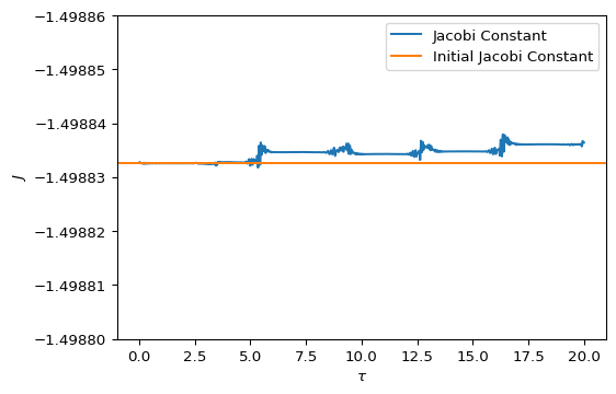
Fig. 24 The Jacobi constant, \(J\), as a function of non-dimensional time using a solver with reduced tolerances. The horizontal line is the initial value of the Jacobi constant.

As shown in Fig. 24, reducing the tolerances significantly improves the behavior of the solver. The change in \(J\) is now on the order of \(1\times 10^{-5}\), which is acceptable for reasonable lengths of integration time.

Fig. 25 shows the trajectory of \(m\) for both of the solution cases here. The trajectories clearly diverge quite quickly after the simulation starts.

fig, ax = plt.subplots(figsize=(5, 5), dpi=96)

# Plot the orbits
ax.plot(r_hp[:, 0], r[:, 1], "r", label="Reduced Tolerances Trajectory")
ax.axhline(0, color="k")
ax.plot(np.hstack((x_2, x_2[::-1])), np.hstack((y_2, -y_2[::-1])))
ax.plot(-pi_2, 0, "bo")
ax.plot(1 - pi_2, 0, "go")
ax.plot(x_0, y_0, "ro")
ax.plot(r[:, 0], r[:, 1], "C2", label="Original Trajectory")
ax.set_aspect("equal")

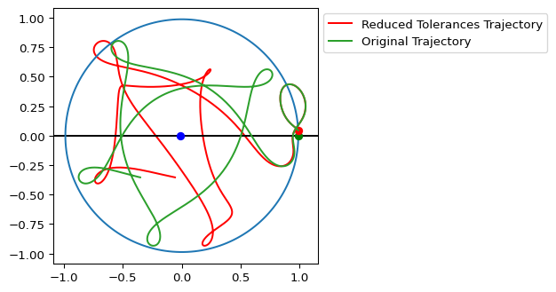
Fig. 25 The two trajectories for the solutions to this problem, in the co-rotating frame.

Cause of Error

Now, let’s examine Fig. 23 and Fig. 24 again. There appears to be a structure to the changes in \(J\). This gives us a hint that the problem might be related to the physical situation that the tertiary mass finds itself in. Let’s plot the distance from the larger mass, given by \(\sigma\), on the same plot as the Jacobi constant.

fig, J_ax = plt.subplots(figsize=(6, 4), dpi=96)
Jacobi_plot = J_ax.plot(sol_hp.t, J_hp, label="Jacobi Constant")
initial_Jacobi = J_ax.axhline(J_hp[0], color="C1", label="Initial Jacobi Constant")
s_ax = J_ax.twinx()
sigma_plot = s_ax.plot(sol_hp.t, sigma_hp, "C2", label=r"$\sigma$")
s_ax.set_ylim(0, 1.15)
J_ax.ticklabel_format(style="plain", useOffset=False)
J_ax.set_xlabel("$\\tau$")
J_ax.set_ylabel("$J$")
s_ax.set_ylabel("$\\sigma$")

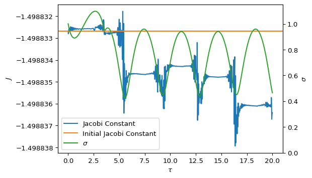
Fig. 26 The Jacobi constant, \(J\), and the non-dimensional position relative to \(m_1\), plotted as a function of non-dimensional time.

As you can see in Fig. 26, the error in the Jacobi constant spikes when the tertiary mass gets closer to the primary mass, \(m_1\). This makes a certain amount of sense, because the acceleration terms depend inversely on the cube of \(\sigma\). As the value of \(\sigma\) gets smaller, the error grows.

This error can be avoided by using a different class of numerical integrators, called symplectic integrators. We won’t have time to discuss those further right now, though. If you’re interested in taking a crack at an implementation, you can find sample code here: http://www.unige.ch/~hairer/software.html, and you will be interested in the Structure-Preserving Algorithms.