

Planetary Ephemeris#
To design realistic interplanetary missions, we must be able to determine the state vector of the relevant planets at a given time, or over a given time interval. This allows calculation of, for instance, the phase angle between planets to determine the window of time to reach the target planet.
The data that gives the state vector are called planetary ephemerides. Due to the chaotic nature of the orbits of the planets, we can only accurately predict planetary state vectors for a relatively short time into the future, about 50–100 years. The chaotic nature of the orbits is due to the complex interaction of the orbits with the gravitational potential from the Sun and Jupiter, primarily.
Ephemerides are also available for more minor objects in the solar system, such as planetary moons and asteroids. The uncertainty over long time intervals of these objects is even higher than for planets, because more objects have the ability to change the orbit of the smaller bodies.
There are several ways to calculate ephemerides. We will discuss three of them here:
Using simplified formulas from JPL
Using more accurate equations with a purpose-built library
Using the online HORIZONS database
In all three cases, we rely on knowing the Julian Day of interest.
Simplified Formulas for Ephemerides#
The simplified formulas for ephemerides from JPL are due to E.M. Standish, and are available from the JPL website. The calculation procedure is further described in the accompanying PDF document.
The simplified formulas give the classical Keplerian orbital elements (\(h\), \(e\), \(M\), \(\nu\), \(\Omega\), and \(\omega\)) for each of the planets. Each element is given with its absolute value at a reference point in time, plus the rate of change of that element. The rates of change are all given per century, and the reference point is the J2000.0 epoch (January 1, 2000 at 12:00 PM (noon) UTC).
The first step is to determine the Julian Date given the Gregorian date and time, with the procedure described in the last section. With that completed, we will need to compute the number of Julian centuries that have elapsed since J2000.0 until the target date. We can do that by:
where \(\mathrm{JDT}\) is the desired Julian Date. Note that this should be floating point division, not integer division.
Next, we need to inspect the data. There are two tables given, one that is valid from AD 1800 to AD 1950, and the other that is valid from 3000 BC to AD 3000. The longer time range has a larger error relative to historical data.
\(a\) [AU, AU/Cy] |
\(e\) [rad, rad/Cy] |
\(i\) [deg, deg/Cy] |
\(L\) [deg, deg/Cy] |
\(\varpi\) [deg, deg/Cy] |
\(\Omega\) [deg, deg/Cy] |
|
|---|---|---|---|---|---|---|
Mercury |
0.38709927 |
0.20563593 |
7.00497902 |
252.250324 |
77.4577963 |
48.3307659 |
0.00000037 |
0.00001906 |
-0.0059475 |
149472.674 |
0.16047689 |
-0.1253408 |
There are 6 columns and two rows associated with each planet. The first row gives the absolute value of the orbital element at the J2000.0 epoch and the second row gives the rate of change of the orbital element. Cy stands for an astronomical century (100 Julian years), or 36,525 days, although this notation is outdated. The six columns are:
Semimajor axis of the orbit (\(a\)), in Astronomical Units, equal to 149,597,870,700 m
Eccentricity (\(e\)), in radians
Inclination (\(i\)), in degrees
Mean Longitude (\(L\)), in degrees
Longitude of perihelion (\(\varpi\)), in degrees
Longitude of the ascending node (\(\Omega\)), in degrees
The coordinates are all given relative to the mean ecliptic plane, and use the vernal equinox of the J2000.0 epoch as the direction of the \(X\) axis, for the purpose of defining 0° longitude.
Once we know the desired time relative to the J2000.0 epoch, in astronomical centuries, the value of any of the parameters given in the table can be found by:
where \(Q\) is any of the properties given in the table, \(\dot{Q}\) is the rate of change of that property, and \(Q_0\) is the initial value at J2000.0. The next steps convert the mean longitude and longitude of the perihelion to the more familar true anomaly and argument of perihelion, respectively.
First, we will calculate the true anomaly using the mean longitude and longitude of perihelion. The mean longitude is related to the mean anomaly by:
The mean anomaly must be in the range of 0-2\(\pi\) radians, so it may be necessary to take the modulus of the result of this equation with 2\(\pi\) to do that. Once the mean anomaly is known, we can use it and the eccentricity to solve Kepler’s equation for the eccentric anomaly, \(E\), using Newton iteration:
The eccentric anomaly can then be used to calculate the true anomaly:
Finally, we can calculate the argument of perihelion from the longitude of perihelion and the longitude of the ascending node:
We now have \(a\), \(e\), \(i\), \(\Omega\), \(\omega\), and \(\nu\), from which we can also calculate \(h\) if necessary. In addition, we can convert the classical orbital elements to a state vector \(\vector{r}\) and \(\vector{v}\) for the planet, if needed.
The data shown in Table 12 are valid from AD 1800-AD 2050. If the data for 3000 BC-AD 3000 are used instead, there are a few extra terms, given in Table 13, which must be used in the equation for the mean anomaly, for the planets from Jupiter to Pluto.
\(b\) |
\(c\) |
\(s\) |
\(f\) |
|
|---|---|---|---|---|
Jupiter |
-0.00012452 |
0.06064060 |
-0.35635438 |
38.35125000 |
The modified equation for the mean anomaly is:
where \(b\), \(c\), \(f\), and \(s\) are from the table, and \(T\) is the desired time. This is the only change necessary between the AD 1800-AD 2050 and the 3000 BC-AD 3000 data.
Let’s calculate the orbital elements for Mercury on December 8, 2020 at 4:30 PM Eastern US time.
from scipy.optimize import newton
from datetime import datetime, timezone
import numpy as np
mercury = {
    "a": 0.38709927, "a_dot": 0.00000037,
    "e": 0.20563593, "e_dot": 0.00001906,
    "i": 7.00497902, "i_dot": -0.0059475,
    "L": 252.250324, "L_dot": 149472.674,
    "long_peri": 77.4577963, "long_peri_dot": 0.16047689,
    "long_node":48.3307659, "long_node_dot": -0.1253408,
}
T_eph = datetime(month=12, day=8, year=2020, hour=21, minute=30, tzinfo=timezone.utc)
We start by defining the data for Mercury from Standish and then creating the datetime object at the appropriate time.
JDT = gregorian_to_julian_date(T_eph)
T = (JDT - 2_451_545) / 36_525
Then, we use the functions defined in Julian Day to calculate the time since the J2000.0 epoch. The JDT is 2,459,192.3958 and the number of centuries since the epoch is 0.2094. Finally, we can calculate the orbital elements.
a = (mercury["a"] + mercury["a_dot"] * T) * 149_597_870.7
e = mercury["e"] + mercury["e_dot"] * T
i = np.radians(mercury["i"] + mercury["i_dot"] * T)
L = np.radians(mercury["L"] + mercury["L_dot"] * T)
long_peri = np.radians(mercury["long_peri"] + mercury["long_peri_dot"] * T)
long_node = np.radians(mercury["long_node"] + mercury["long_node_dot"] * T)

M_e = (L - long_peri) % (2 * np.pi)
def kepler(E, M_e, e):
    """Kepler's equation, to be used in a Newton solver."""
    return E - e * np.sin(E) - M_e

def d_kepler_d_E(E, M_e, e):
    """The derivative of Kepler's equation, to be used in a Newton solver.

    Note that the argument M_e is unused, but must be present so the function
    arguments are consistent with the kepler function.
    """
    return 1 - e * np.cos(E)

E = newton(func=kepler, fprime=d_kepler_d_E, x0=np.pi, args=(M_e, e))
nu = (2 * np.arctan(np.sqrt((1 + e) / (1 - e)) * np.tan(E / 2))) % (2 * np.pi)

omega = long_peri - long_node

print(f"𝑎 = {a:.5G} km", f"𝑒 = {e:.5F}", f"𝑖 = {np.degrees(i):.2F}°", f"𝜃 = {np.degrees(nu):.2F}°",
      f"𝜔 = {np.degrees(omega):.2F}°", f"𝛺 = {np.degrees(long_node):.2F}°", sep="\n")
𝑎 = 5.7909E+07 km
𝑒 = 0.20564
𝑖 = 7.00°
𝜃 = 159.93°
𝜔 = 29.19°
𝛺 = 48.30°
Using a Library for Ephemerides#
The formulas given in the last section are only approximate, with errors up to a few thousand kilometers, depending on the time interval and the particular planet of interest. JPL also produces much higher accuracy ephemerides (errors on the order of centimeters to a few kilometers) which are included in some specialized software. One example of such software available for Python is called poliastro, which we’ll be using here. There are several other options as well:
pyEphem (outdated and replaced by the next item)
Astropy (also used by poliastro for some computations)
All these libraries use either the NASA SPICE database, in the form of SPK files, or the NASA/JPL HORIZONS database, which we’ll also discuss in the next section.
poliastro has a number of methods to produce ephemerides for the planets and also has a convenient interface to retrieve the classical orbtial parameters, which is why I’ve selected it here. The two main methods are:
Lower-accuracy Astropy ephemerides, which rely on the PyERFA library
Higher-accuracy JPL ephemerides using the SPICE files
The Astropy ephemerids are included when poliastro is installed, while the JPL ephemerides require a separate download. We’ll use the JPL ephemerides in this example. First, we need to determine a time at which the ephemerides should be calculated. poliastro requires an instance of the Astropy time.Time() class to work, but we can create that using the datetime we set in the last section.
from astropy import time
epoch = time.Time(T_eph)
Next, we will set Astropy to use the JPL ephemerides.
from astropy.coordinates import solar_system_ephemeris
solar_system_ephemeris.set("jpl")
Then, we’ll compute the ephemerides using poliastro.
from poliastro.ephem import Ephem
from poliastro.bodies import Sun, Mercury
from poliastro.twobody import Orbit
merc_ephem = Ephem.from_body(Mercury, epoch.tdb)
merc_orbit = Orbit.from_ephem(Sun, merc_ephem, epoch)
print(f"𝑎 = {merc_orbit.a:.5G}", f"𝑒 = {merc_orbit.ecc:.5F}", f"𝑖 = {merc_orbit.inc.to('degree'):.2F}",
      f"𝜃 = {merc_orbit.nu.to('degree'):.2F}", f"𝜔 = {merc_orbit.argp.to('degree'):.2F}",
      f"𝛺 = {merc_orbit.raan.to('degree')}", sep="\n")
𝑎 = 5.7567E+07 km
𝑒 = 0.20149
𝑖 = 28.64 deg
𝜃 = 164.05 deg
𝜔 = 62.56 deg
𝛺 = 10.790248210752855 deg
The parameters of the orbit are listed in the poliastro documentation: https://docs.poliastro.space/en/stable/autoapi/poliastro/twobody/index.html#poliastro.twobody.Orbit.
Notice that the inclination is significantly different from the inclination we calculated previously. This is due to the plane of the orbit that we defined. By default, poliastro uses the Earth-equatorial reference frame, which is inclined relative to the ecliptic plane.
print(merc_orbit.plane)
Planes.EARTH_EQUATOR
To change the plane to the ecliptic, we must change the plane when we create the ephemerides:
from poliastro.frames import Planes

merc_ephem = Ephem.from_body(Mercury, epoch.tdb, plane=Planes.EARTH_ECLIPTIC)
merc_orbit = Orbit.from_ephem(Sun, merc_ephem, epoch)
print(merc_orbit.plane, f"𝑖 = {merc_orbit.inc.to('degree'):.2F}", sep="\n")
Planes.EARTH_ECLIPTIC
𝑖 = 7.01 deg
As you can see, we now have the Earth ecliptic as the reference plane, and the inclination matches the previous calculation. The other major difference is in the true anomaly. This is due to the default choice of the reference point as the solar system barycenter. We can adjust the default reference point, which again we must do when we create the ephemerides. We do this by setting the attractor parameter for the ephemerides:
merc_ephem = Ephem.from_body(Mercury, epoch.tdb, attractor=Sun, plane=Planes.EARTH_ECLIPTIC)
merc_orbit = Orbit.from_ephem(Sun, merc_ephem, epoch)
print(f"𝜃 = {merc_orbit.nu.to('degree'):.2F}")
𝜃 = 159.93 deg
Now the result is much closer to the one we calculated previously.
Matlab has a similar function, called planetEphemeris. You have to install the Aerospace Toolbox, for which instructions can be found on the Mathworks website or you can click the “Add-Ons” button in the Matlab ribbon toolbar and search for “aerospace toolbox”. The first time you run planetEphemeris, it will also prompt you to install the SPK files to do the calculations.
With that all installed, planetEphemeris takes 3 arguments in the basic form:
A Julian Date
The center of the desired coordinate system
The target object
planetEphemeris then returns the position and velocity vector with respect to the center that you set. The default units are km and km/s.
t1 = datetime('2020-December-08 21:30');
t1.TimeZone = 'UTC';
jd1 = juliandate(t1);
[position, velocity] = planetEphemeris(jd1, 'Sun','Mercury','432t');
angular_momentum = cross(position, velocity);
h = norm(angular_momentum);
i = acos(angular_momentum(end) / h);
rad2deg(i)

ans =

   28.5532
Once the position and velocity are obtained, we can use the methods from Classical Orbital Elements and the State Vector to convert to the classical orbital elements.
Note that the inclination is about 28 degrees, meaning that the default frame is the Earth-equatorial frame, equivalent to the ICRF. We can convert from this frame to the ecliptic frame by a rotation around the vernal equinox:
where \(\varepsilon\) is the obliquity of the ecliptic and \(Q\) is the rotation matrix. The current value of \(\varepsilon\) is 23.43657°. Thus, the transformation is accomplished by:
obliquity = deg2rad(23.43657);
transform = [1 0 0; 0 cos(obliquity) sin(obliquity); 0 -sin(obliquity) cos(obliquity)];
pos = transform * position';
vel = transform * velocity';
am = cross(pos, vel);
h2 = norm(am);
rad2deg(acos(am(end) / h2))

ans =

    7.0055
With this coordinate transformation, we obtain the same inclination angle as before.
Using JPL HORIZONS Web Interface#
JPL also maintains a web browser based interface to the HORIZONS database. This interface can be used to determine all the same information as the previous methods, with a similar level of accuracy as the SPICE-focused methods in the previous section. The web interface is located at:
https://ssd.jpl.nasa.gov/horizons/app.html#/
The default interface of HORIZONS is shown in Fig. 95
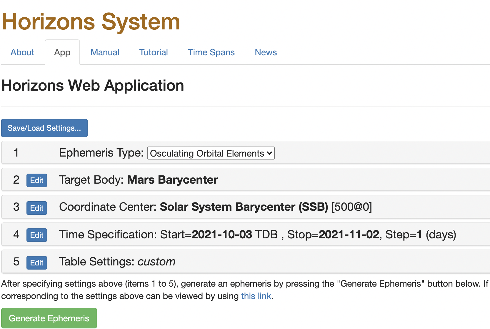
Fig. 95 The default web interface for HORIZONS.#
Each of the options can be changed by clicking the Edit buttons. For our purposes, we can change the following:
Ephemeris Type: Either Vector Table or Osculating Orbital Elements is suitable, although the latter is more direct for this example
Target Body: This option opens a pop-up where we can search for the body of interest. In the drop-down menu under Choose a method for specifying the target body, you can choose Select from a list of major bodies, then choose Mercury
Center: The default selection here is Solar System Barycenter, the center of gravity of the entire solar system. This is usually a little bit outside the Sun, depending on the relative locations of the planets, especially Jupiter. In our case, we want the center of the Sun as the focus of the orbit, so click Edit and then type
@suninto the search box.Time Span: This can be used to generate a range of dates, or to input specific dates. We will choose Specify a list of times for this example, and then input the date of interest, in JDT, 2,459,192.3958.
Table Settings: Here, we want to change the units to km and seconds. Another useful option is the Reference plane. The default of ecliptic x-y plane derived from reference plane is appropriate for this example. You may also want to set the CSV output option, depending on how you will use the data.
When you’ve set the options for this example, the screen should appear as in Fig. 96.
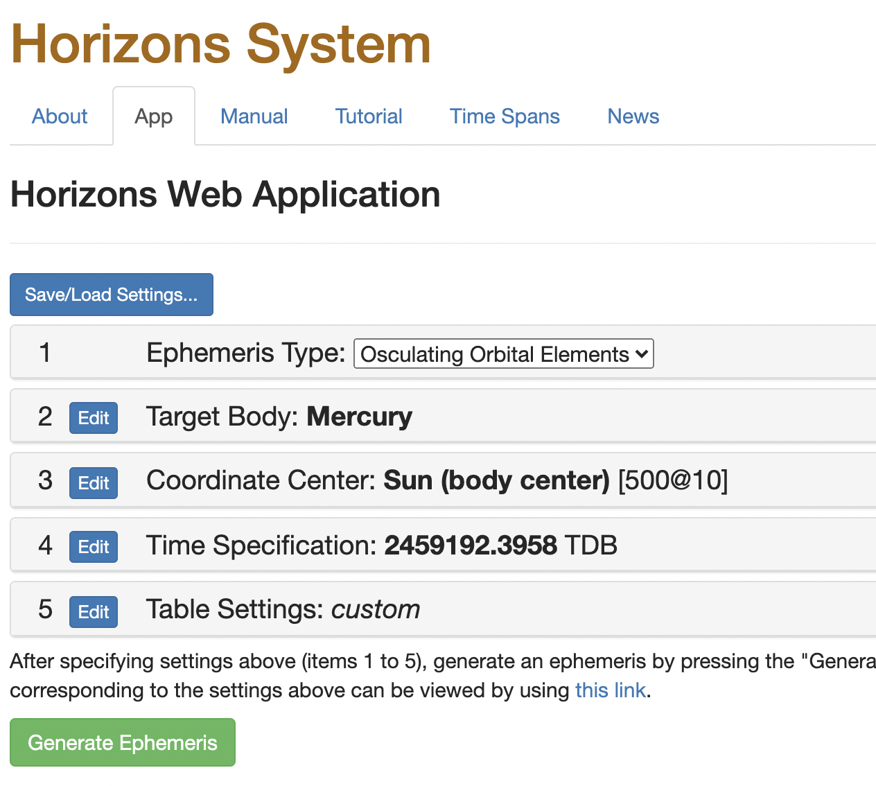
Fig. 96 The settings used in this example for the ephemerides of Mercury.#
After clicking Generate Ephemeris, the output looks like Fig. 97.
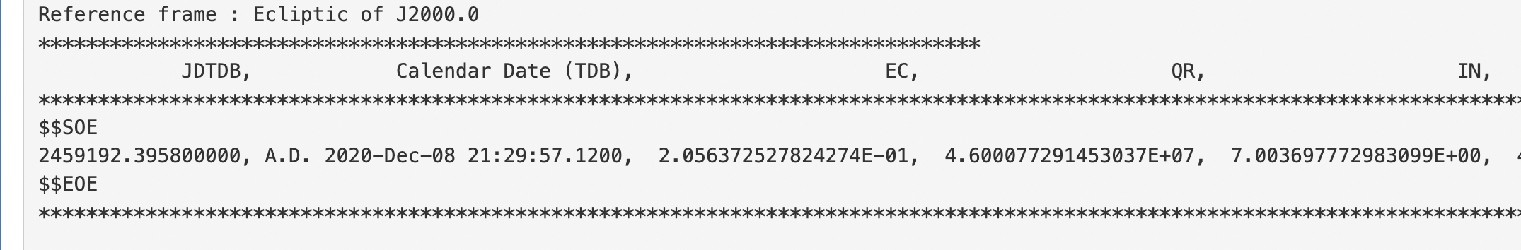
Fig. 97 A subset of the output from HORIZONS for Mercury showing the orbital elements.#
The HORIZONS output includes data about Mercury itself, the dates for which the ephemeris were calculated, and as shown in Fig. 97, the orbital elements of interest. Right below the orbital elements output is an explanation of what the acronyms mean. IN stands for inclination and TA is the true anomaly. Both of these elements match our previous calculated results for the date given.