Application of the CR3BP: Lagrange Points

The equations of motion of the circular restricted three body problem (CR3BP) were shown in Eq. (71). These non-dimensional equations of motion do not have a general analytical solution.

Lagrange himself called them libration points so you will see them called that too.

However, there are a set of five points for which the tertiary mass is in equilibrium with respect to the primary and secondary masses. An object placed at one of the equilibrium points will, if it is not perturbed, remain at that location indefinitely. These locations are called Lagrange Points.

According to the conditions for equilibrium, the acceleration and velocity components at the Lagrange points are zero:

(72)\[\dot{x}^* = \dot{y}^* = \dot{z}^* = 0 \qquad \text{and} \qquad \ddot{x}^* = \ddot{y}^* = \ddot{z}^* = 0\]

and likewise for the dimensional coordinates as well. Plugging these conditions in to the equations of motion, we find:

(73)\[\begin{split}\begin{aligned} -x^* &= -\frac{1 - \pi_2}{\sigma^3}\left(x^* + \pi_2\right) - \frac{\pi_2}{\psi^3}\left(x^* - 1 + \pi_2\right) \\ -y^* &= -\frac{1 - \pi_2}{\sigma^3} y^* - \frac{\pi_2}{\psi^3}y^* \\ 0 &= \left(-\frac{1 - \pi_2}{\sigma^3} - \frac{\pi_2}{\psi^3}\right)z^* \end{aligned}\end{split}\]

In the last equation, for \(z^*\), the terms in the parentheses are both greater than zero. Therefore, there is no way for them to cancel each other out, and the only way for the equation to be satisfied is if \(z^* = 0\). Thus, the Lagrange points lie in the orbital plane.

Now, we need to solve for the \(x^*\) and \(y^*\) coordinates of the Lagrange points. There are two conditions that we need to consider, since they end up with different solutions:

1. \(y^* \neq 0\), giving the so-called equilateral Lagrange points

2. \(y^* = 0\), giving the so-called collinear Lagrange points

The collinear Lagrange points lie along the \(x^*\) axis, between \(m_1\) and \(m_2\). The equilateral Lagrange points form an equilateral triangle with \(m_1\) and \(m_2\) as two of the corners and sides of length \(r_{12}\).

Equilateral Lagrange Points

Remember that \(z^*\) is zero for all the equilibrium points.

To find the equilateral Lagrange points, we assume \(y^*\neq 0\). Now we have 2 equations and 2 unknowns. Since \(y^*\neq 0\), the \(y^*\) in the second equation of motion (Eq. (73)) will cancel from both sides, and we end up with:

(74)\[1 = \frac{1 - \pi_2}{\sigma_3} + \frac{\pi_2}{\psi^3}\]

The equation for \(x^*\) in Eq. (73) we see the \(\left(1 - \pi_2\right)/\sigma^3\) term, so let’s solve the \(y^*\) equation for that and plug into the \(x^*\) equation:

(75)\[x^{*} = \left(1 - \frac{\pi_2}{\psi^3}\right)\left(x^* + \pi_2\right) + \frac{\pi_2}{\psi^3}\left(x^* - 1 + \pi_2\right)\]

Simplifying, we find:

(76)\[\psi^3 = 1\]

Then we can use the definition of \(\psi\) to find \(r_2\) in dimensional coordinates:

(77)\[\psi = \frac{\mag{\vector{r}*2}}{r*{12}} \Rightarrow r_2 = r_{12}\]

Plugging the result of Eq. (76) back into Eq. (74) equation, we find:

(78)\[\sigma^3 = 1\]

Then we can use the definition of \(\sigma\) to find \(r_1\) in dimensional coordinates:

(79)\[\sigma = \frac{\mag{\vector{r}*1}}{r*{12}} \Rightarrow r_1 = r_{12}\]

Since if \(a = b\) and \(b = c\), then \(a = c\), we find:

(80)\[r_1 = r_2 = r_{12}\qquad \text{and}\qquad \psi = \sigma\]

for the equilateral Lagrange points. Eq. (80) shows that the distance from \(m_1\) to \(m\) is the same as the distance from \(m_2\) to \(m\) and from \(m_1\) to \(m_2\). This defines an equilateral triangle, giving these Lagrange points their name.

From the definition of \(\vector{\sigma}\) and \(\vector{\psi}\), we can take their magnitudes and equate them to solve for the values of \(x^*\) and \(y^{*}\) at the equilibrium points:

(81)\[\begin{split}\begin{aligned} \sigma^2 &= \mag{\vector{\sigma}}^2 = \left(x^{*} + \pi_2\right)^2 + \left(y^*\right)^2 \\ \psi^2 &= \mag{\vector{\psi}}^2 = \left(x^{*} - 1 + \pi_2\right)^2 + \left(y^*\right)^2 \end{aligned}\end{split}\]

where we have also used the fact that \(z^* = 0\) for the Lagrange points. Using the result from Eq. (80) that \(\sigma = \psi\) for the equilateral points, we find:

(82)\[\begin{split}\begin{aligned} x^{*} &= \frac{1}{2} - \pi_2 \\ y^* &= \pm \frac{\sqrt{3}}{2} \end{aligned}\end{split}\]

The equilateral Lagrange points are given the symbols \(L_4\) and \(L_5\), for the positive and negative \(y^*\) values, respectively:

(83)\[\begin{split}\begin{aligned} &L_4: & x^* &= \frac{1}{2} - \pi_2 & y^*&= \frac{\sqrt{3}}{2} \\ &L_5: & x^* &= \frac{1}{2} - \pi_2 & y^*&= -\frac{\sqrt{3}}{2} \end{aligned}\end{split}\]

To convert these to dimensional \(x\) and \(y\) coordinates, you should multiply by \(r_{12}\).

Collinear Lagrange Points

For the collinear Lagrange points, we set \(y = z = y^{*} = z^* = 0\) in the equations of motion, Eq. (71). We make this choice by inspection, seeing that setting \(y = y^{*} = 0\) is one possible solution (the other case, \(y^*\neq 0\) we just handled).

This leaves only the \(x^*\) equation of motion, since the other two are trivially \(0=0\). For \(x^*\), we have from Eq. (73):

(84)\[x^{*} = \frac{1 - \pi_2}{\sigma^3}\left(x^* + \pi_2\right) + \frac{\pi_2}{\psi^3}\left(x^* - 1 + \pi_2\right)\]

The vectors \(\vector{\sigma}\) and \(\vector{\psi}\) are the non-dimensional versions of the vectors from \(m_1\) and \(m_2\) to \(m\).

The terms \(\sigma^3\) and \(\psi^3\) in the bottom of both terms are found by cubing the magnitude of the vectors \(\vector{\sigma}\) and \(\vector{\psi}\). To find the vector magnitude, we necessarily have to take the square root, so we do not know the sign of the magnitude. Cubing a negative number will result in another negative and cubing a positive number will result in another positive.

Therefore, we do not know what the sign of \(\sigma^3\) or \(\psi^3\) will be, we have to include that as part of the solution of this equation. Cubing the magnitudes of \(\vector{\sigma}\) and \(\vector{psi}\) from Eq. (66) with \(y^* = 0\) for the collinear points, we find:

(85)\[\begin{aligned} \sigma^3 &= \left\lvert x^{*} + \pi_2\right\rvert ^3 & \psi^3 &= \left\lvert x^* - 1 + \pi_2\right\rvert ^3 \end{aligned}\]

where the single vertical lines indicate that we’re taking the absolute value. Substituting these into Eq. (84), we find:

(86)\[0 = x^{*} - \frac{1 - \pi_2}{\left\lvert x^* + \pi_2\right\rvert ^3}\left(x^* + \pi_2\right) - \frac{\pi_2}{\left\lvert x^* - 1 + \pi_2\right\rvert ^3}\left(x^* - 1 + \pi_2\right)\]

We cannot cancel any of the terms because we don’t know the sign of the cubic term on the bottom.

This equation is cubic in \(x^*\), so it will have three separate values of \(x^*\) that solve the equation, as long as \(0 < \pi_2 < 1\). In the cases where \(\pi_2 = 0\) or \(\pi_2 = 1\), either \(m_2\) or \(m_1\) must be zero, which aren’t very interesting.

There is no analytical solution to this equation, it must be solved numerically. There are many methods to solve the equation numerically, my suggestions are to use scipy.optimize.newton() in Python and fzero in Matlab. We will see how to use these functions in the next example.

In the meantime, Fig. 15 shows the solution of Eq. (86):

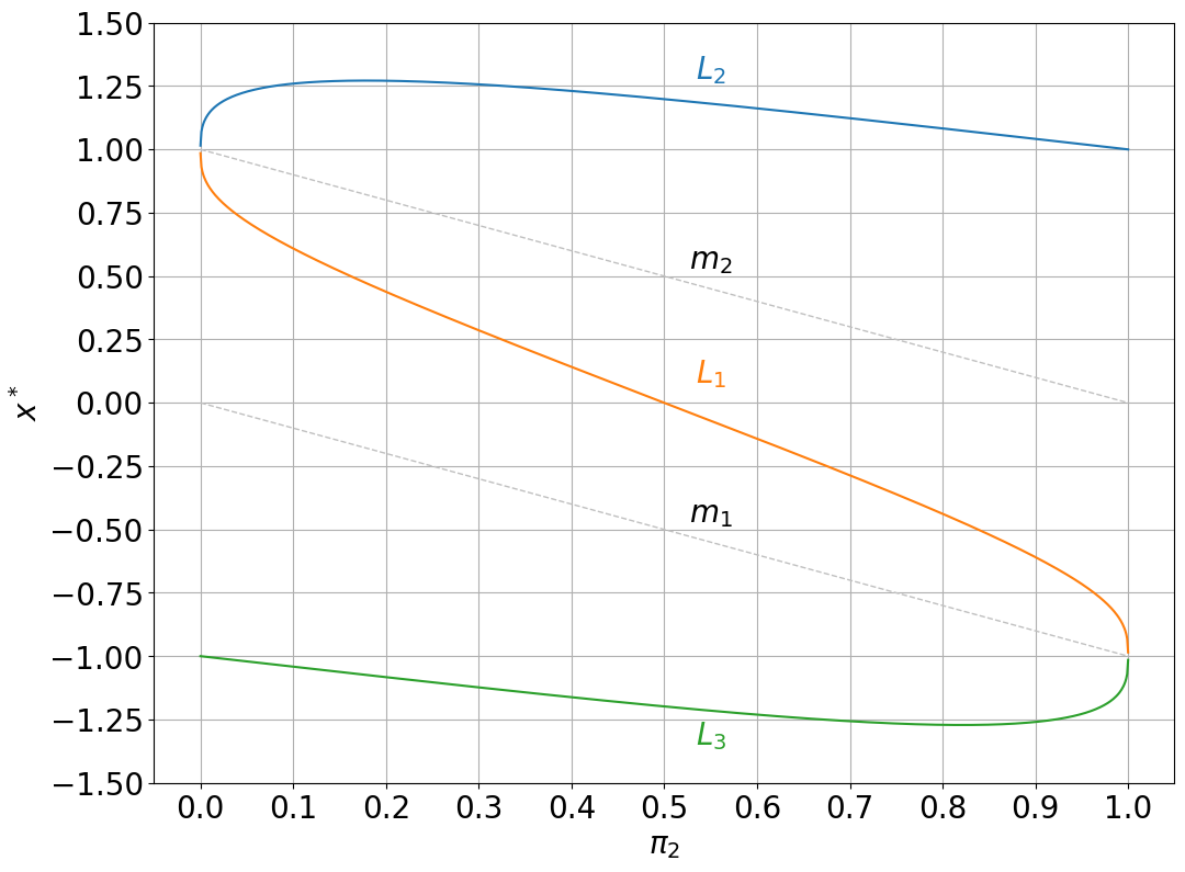
Fig. 15 The solutions of Eq. (86), showing the dimensionless positions of the collinear Lagrange points as a function of the dimensionless mass.

On this figure, the \(x\) axis is \(\pi_2\) and the \(y\) axis is \(x^*\). For a given value of \(\pi_2\), we can locate the three values of \(x^*\) that solve the equation. The gray dashed lines give the corresponding positions of \(m_1\) and \(m_2\) at the given value of \(\pi_2\).

The solutions for \(x^*\) for the collinear Lagrange points lie on the S-curve shape. For a given value of \(\pi_2\), we can see there are 3 solutions of the function, corresponding to the three collinear Lagrange points for that system.

By convention, the Lagrange points are numbered such that \(L_1\) lies between \(m_1\) and \(m_2\), \(L_2\) lies to the right of \(m_2\), and \(L_3\) lies to the left of \(m_1\). Thus, we can see on the figure that the upper part of the S-curve is the solution for \(L_2\). Below \(x^{*} = 1.0\), the solution is for \(L_1\), since that lies between \(m_1\) and \(m_2\). Finally, below \(x^{*} = -1.0\), the solution is for \(L_3\).

Fig. 16 plots the five Lagrange points in non-dimensional coordinates as a function of the mass ratio \(\pi_2\).

Once Loop Reflect

Fig. 16 Animation showing the position of the five Lagrange points as the value of \(\pi_2\) goes from 0 to 1.

Fig. 16 shows that the solution of the equations of motion for the equilibrium points is symmetrical. We chose \(m_1\) to be the larger mass at the start of the problem, but we can interchange \(m_1\) and \(m_2\) without any problems.

For the Earth-Moon system, the value of \(\pi_2\) is approximately 0.012.

Lagrange Point Stability

Although all the Lagrange points are equilibrium points, they may not be stable equilibrium points. Stability is the ability of the system to return to its initial position after being perturbed.

To analyze the stability of the Lagrange points, we will use the potential energy function for the CR3BP.

As we discussed previously, gravity is a conservative force. As such, the force field can be defined in terms of a potential energy function. For the CR3BP, the pseudo-potential function in the rotating frame is given by Koon et al. [KLMR11]:

(87)\[U(x^*, y^*) = -\frac{1 - \pi_2}{\sigma} - \frac{\pi_2}{\psi} - \frac{1}{2}\left[\left(1 - \pi_2\right)\sigma^2 + \pi_2 \psi^2\right]\]

A plot of this function is shown in Fig. 17, including the positions of the five Lagrange points, for \(\pi_2 =\) 0.3.

Fig. 17 The pseudo-potential energy function in the rotation reference frame used for the CR3BP, with \(\pi_2 =\) 0.3. The five Lagrange points for this system are labeled on the figure.

Using this figure, we can get a qualitative sense of the stability of the Lagrange points. Imagine that we turn the potential function upside-down, and put a marble on each of the Lagrange points.

We can see that \(L_4\) and \(L_5\) are at the bottom of a bowl. Slight displacements of the marble will cause it to return to the initial position, so these points are considered stable Lagrange points.

On the other hand, \(L_1\), \(L_2\), and \(L_3\) are saddle points on the potential energy surface. This means that slight displacements will cause the object’s position to diverge from the equilibrium point over time.

The Equilateral Lagrange Points

Since the equilateral Lagrange points are stable, objects placed in a small orbit, usually called a halo orbit, around those points will tend to remain there. The criterion for stability is:

(88)\[\frac{m_1}{m_2} + \frac{m_2}{m_1} \geq 25\]

Note that Fig. 17 shows the potential surface for \(\pi_2 = 0.3\), which does not satisfy the numerical stability criteria here for \(L_4\) and \(L_5\) from Eq. (88). We’re plotting \(\pi_2 = 0.3\) to exaggerate the shape of the potential function for clarity.

which will be satisfied if \(m_1/m_2>24.95994\) or \(\pi_2 < 0.0385209\). In the Earth-Moon system, that ratio is \(m_1/m_2 \approx 81.3\), so \(L_4\) and \(L_5\) are nominally stable. However, the \(L_4\) and \(L_5\) points for the Earth-Moon system are slightly destabilized by the influence of the sun and they aren’t completely stable. Nonetheless, there are clouds of dust which have collected at these points because they are kinda stable.

Other pairs of \(m_1\) and \(m_2\) do have somewhat more stable \(L_4\) and \(L_5\) points. In particular, the orbit of Jupiter around the sun has stable equilateral Lagrange points. There are groups of asteroids, called Trojan asteroids that cluster around the stable Lagrange points in the orbit of Jupiter, as shown in Fig. 18.

Fig. 18 The Trojan and the Greek asteroids are clusters of asteroids that have collected at the stable \(L_4\) and \(L_5\) Lagrange points in the Sun-Jupiter system.

The Collinear Lagrange Points

The collinear Lagrange points, \(L_1\), \(L_2\), and \(L_3\) are all saddle points in Fig. 17, meaning that the function increases when going in one axis, but decreases going in the other axis. This means that the three collinear Lagrange points are unstable and an object placed at one of those points, if perturbed, will diverge from the position.

Nonetheless, these are quite useful points for observation of the solar system. Several satellites have been placed at the \(L_1\) point of the Earth-Sun system for solar observation, and the James Webb Space Telescope (JWST) is located at the \(L_2\) point in the Earth-Sun system specifically to avoid sunlight interefering with observations.

These satellites orbit around the unstable Lagrange points in a Lissajous orbit. This type of orbit requires a very small amount of propulsion onboard the satellite to keep position, but the orbit can last for a very long time with only a little fuel. One example is the Wilkinson Microwave Anisotropy Probe (WMAP) which was sent to the \(L_2\) point in the Earth-Sun system to study the Cosmic microwave background. The trajectory of WMAP is shown in Fig. 19.

Fig. 19 The trajectory of the Wilkinson Microwave Anisotropy Probe (WMAP) as viewed from Earth. Note the distance in the bottom of the animation, showing the satellite as approximately 1.5 million km from the earth. Phoenix7777, CC BY-SA 4.0, via Wikimedia Commons.

Another example is the JWST, mentioned previously. JWST has a simpler halo orbit around \(L_2\). The orbit of JWST is shown in Fig. 20.

Fig. 20 The trajectory of the James Webb Space Telescope (JWST) as viewed from above the ecliptic plane with Earth fixed. Note again the distance in the bottom of the animation, showing the satellite as approximately 1.5 million km from the earth. Phoenix7777, CC BY-SA 4.0, via Wikimedia Commons.

\(L_1\) and \(L_2\) in the Earth-Sun system are about 1.5 million km towards the Sun and away from the Sun, starting at the Earth, respectively. \(L_3\) lies on the other side of the Sun, and has long been the predicted location of a hidden planet, since it could not be observed from Earth prior to the advent of satellite observation. Now, of course, we know there is no planet at that location.